")
")
| Issue |
Sci. Tech. Energ. Transition
Volume 80, 2025
|
|
|---|---|---|
| Article Number | 18 | |
| Number of page(s) | 22 | |
| DOI | https://doi.org/10.2516/stet/2024109 | |
| Published online | 29 January 2025 | |
Regular Article
A framework for optimisation and techno-economic analysis of CO2 pressurisation strategies for pipeline transportation
1
Process Department, Energy Transition, Ramboll Energy, Bavnehøjvej 5, Esbjerg, DK-6700, Denmark
2
ORS Consulting, Borgergade 66 st. th, Esbjerg, DK-6700, Denmark
* Corresponding author: This email address is being protected from spambots. You need JavaScript enabled to view it.
, This email address is being protected from spambots. You need JavaScript enabled to view it.
Received:
16
April
2024
Accepted:
19
December
2024
Abstract
This paper presents a framework for optimisation and techno-economic analysis of various pressurisation pathways for CO2 pipeline transportation. The pressurisation pathways include a conventional compression only case from initial to final pressure, a sub-critical compression part followed by cooling, liquefaction and pumping and also a super-critical compression part followed by cooling and dense phase pumping. The presented framework is developed based on open-source components and information available in the public domain. The framework includes a high level of flexibility to study variations in intial and final pressures, inclusion of inter-stage pressure drop, inter-stage cooling temperature, liquefaction/pumping pressure, among others. The implemented methods, i.e., the thermodynamic and economic models applied, are rigorously validated and bench-marked against literature data. Contrary to former studies that focus mainly on reduction of the work required for pressurisation, the presented method includes additional capabilities to assess CAPEX, OPEX and the levelised cost of CO2 compression. The analysis shows that in some cases the minimum levelised cost does not coincide with the minimum work. It is also demonstrated that for some cases the super-critical compression/cooling/pumping case and the sub-critical compression/cooling/liquefaction/pumping pathways provide optimal levelised cost compared to a multi-stage compression only case.
Key words: CCUS / Carbon dioxide compression and pumping / Carbon dioxide liquefaction and transport / Techno-economic analysis / Thermodynamic analysis / Process simulation and optimisation
The affiliation of the corresponding author has changed during the publication process.
© The Author(s), published by EDP Sciences, 2025
 This is an Open Access article distributed under the terms of the Creative Commons Attribution License (https://creativecommons.org/licenses/by/4.0), which permits unrestricted use, distribution, and reproduction in any medium, provided the original work is properly cited.
Abbreviations
A: Area
ACHE: Air Cooled Heat Exchanger
API: American Petroleum Institute
ASME: American Society of Mechanical Engineers
BB: Between Bearings
BPVC: Boiler and Pressure Vessel Code
CAPEX: Capital Expenditure
CEPCI: Chemical Engineering Plant Cost Index
CF: Capacity Factor
COP: Coefficient of Performance
CRF: Capital Recovery Factor
CS: Carbon Steel
DOE (U.S.): Department of Energy
EDF: Enhanced Detailed Factor
EOR: Enhanced Oil Recovery
EPC: Engineering Procurement Construction
EU: European Union
FOB: Free On-Board
FEED: Front End Engineering Design
FOPEX: Fixed Operational Expenditure
GPSA: Gas Processors Suppliers Association
IECM: Integrated Environmental Control Model
LCOCC: Levelised Cost of CO2 Compression
LCOE: Levelised Cost of Electricity
LMTD: Logarithmic Mean Temperature Difference
m: Mass
MEA: Monoethanolamine
MM: Mille Mille
MTD: Mean Temperature Difference
NETL: National Energy Technology Laboratory
O&M: Operations and Maintenance
OEM: Original Equipment Manufacturer
OPEX: Operational Expenditure
P: Pressure or Power
PCC: Post-Combustion (Carbon) Capture
PR: Peng-Robinson
SAF: Sustainable Aviation Fuel
SHE: Shell & Tube Heat Exchanger
SS: Stainless Steel
TPC: Total Plant Cost
USD: U.S. Dollars
VF: Vapour Fraction
VLE: Vapour Liquid Equilibrium
VOPEX: Variable Operational Expenditure
1 Introduction
When captured CO2 from, e.g., post-combustion capture [1] is to be transported from the capture site to a final destination be it for injection into subsurface reservoirs for long-term storage [2], for off-site utilisation into various e-fuels such as e-methanol [3], e-methane or Sustainable Aviation Fuels (SAF), for Enhanced Oil Recovery (EOR) [4] or other means of storage or reuse, high pressure pipeline transport above the critical pressure is found to be the most effective method [5, 6]. To achieve such high pressure, the captured CO2 needs to be pressurised often by a factor of 100 or more. When CO2 is captured, it exits the capture facility in a gaseous state, typically at 1–2 bar pressure for post-combustion capture. Pressurisation via gas compression is a straightforward choice. Provided sufficient compression stages with applied inter-cooling, the pressure eventually reaches the desired value for transport above the critical point. Depending on the available cooling utility and the achievable temperature, this will either result in CO2 in the supercritical or dense phase region. Another option for pressurisation is gas compression to a pressure below the critical pressure, followed by cooling/liquefaction and liquid pumping until the final pressure is reached (in the dense phase region). A variant of this is gas compression to a pressure above the critical point, yet below the final pressure, followed by cooling below the critical temperature and dense phase pumping to the final pressure. Finding the optimal pressurisation pathway has been addressed in several investigations [7–10].
Witkowski and Majkut [7] investigated 13 different CO2 compression concepts for post-combustion capture from a 900 MW pulverised coal-fired power plant including heat integration. All cases considered compression from 1.51 bar to 153 bar. Some of their findings include a reduction in power by increasing the number of compression stages, increasing power with higher inter-stage temperatures, and also that a compression path from the initial pressure to an intermediate pressure followed by liquefaction and pumping to the final pressure offers significant reduction in compression power. However, the authors do not include a quantification of the compression power required for the refrigeration cycle.
Martynov et al. [8] studied three different pressurisation pathways for different CO2-rich streams from pure CO2 and post-combustion capture to increasing content of impurities including pre-combustion capture to different oxy-fuel capture purities. The compression pathways included a multi-stage compression pathway, a shock-wave compression pathway, and a compression/cooling/liquefaction/pumping pathway. All systems considered pressurisation from 15 bar to 151 bar with the latter case including liquefaction and pumping from 62 bar to the final pressure. It was found that compression power increased moderately for increasing impurity levels up to 4 v/v %. Further, increasing impurities up to v/v 15% results in significantly increasing power requirement. The same trend was observed for the required refrigeration compression power for liquefaction at 62 bar.
Dlamini et al. [10] studied different pressurisation pathways for pipeline transport of CO2 including both pure compression and sub-critical compression followed by cooling/liquefaction/pumping to the final delivery pressure. Pressurisation was from 4.6 barg in all cases. The effect of number of compression stages, cooling temperatures, pipeline back-pressure was investigated as well as different heat integration methods. It was concluded that for the compression/liquefaction/pumping pressurisation pathway, a liquefaction pressure of 45 bar was optimal using three compression stages (and a two-stage refrigeration process), whereas a compression only case with eight stages was marginally better when the cooling in inter-stage coolers occurred at 35 °C. When the cooling temperature was lowered to 25 °C and 10 °C, respectively, the subcritical compression/cooling/liquefaction/pumping become energetically more favourable with savings of 10% and 27% in work duty, respectively.
From the review of prior studies it appears as the dependent parameter of primary interest has been the power consumption. To the best of our knowledge, rigorous combined investigations considering a plethora of variables and responses of both technical aspects, such as power consumption, as well as economic aspects, such as Capital Expenditure (CAPEX), Operational Expenditure (OPEX) and levelised cost of pressurisation, is very sparse. One exception being the work of Magli et al. [11], who studied the combined compression and purification of oxy-fuel based capture on cement plants.
Considering the vast amount of parameters that affects the pressurisation pathway, we present a rigorous modelling framework that is flexible and can handle any combination of parameters, like inlet/outlet pressure, pressurisation pathway (compression only or compression, cooling/liquefaction and pumping), cooling temperatures, pressure drop in compression stages, different number of compression stages, all based on open source software. In addition, an integrated approach for estimating equipment and total plant costs that relies on methods and databases openly available and documented is described and applied. Thus, the presented tool does not rely on proprietary closed source black-box models or databases for full transparency and clarity.
2 Methods
2.1 System description and parameters investigated
The main purpose of the simulation program presented in this study is to analyse the compression of CO2 from low to high pressure suitable for pipeline transport. The program is flexible in the sense that the number of compression stages can be specified. The program also includes modelling of liquefaction of CO2 at any pressure below the critical point with subsequent pumping to the final desired pressure. The program calculates required compression power, cooling duty, liquefaction duty as well as refrigeration power (by refrigerant vapour compression) and pumping power. In addition, the program provides CAPEX estimates, OPEX estimates, and it calculates the Levelised Cost of CO2 Compression (LCOCC). This allows a full techno-economic analysis providing a basis for minimizing both energy and levelised cost of transporting CO2.
A schematic process flow diagram visualising the capabilities of the simulation model is shown in Figure 1. The process pressurises carbon dioxide from feed, Pin, to final pressure, Pout. A CO2 stream, either pure or with impurities, delivered at a specified pressure and temperature (Pin, Tfeed) enters a multistage compression process with n number of compression stages. In each stage, the fluid is compressed (isentropic) with a specified isentropic efficiency, ϵ. The discharge of each compression stage is cooled/inter-cooled to a specified temperature Tin, which is the inlet of the succeeding compression stage. The pressure drop, dP, for each compression stage can be specified, and the pressure drop is assigned to the inter-cooler. The number of stages is an integer equal to or larger than 1.
If the pressurisation to the final pressure is selected to be by vapour phase/supercritical compression only, the fluid leaving the last compression stage is routed to export/pipeline at the final specified pressure. However, if the input to the simulation specifies liquefaction before final pressurisation via liquid pumping by specifying a liquefaction pressure Pliq below the critical point, the part of the process named “Cooling, liquefaction and pumping” is activated. The involved streams are thick in the schematic. In that case, the fluid compressed in vapour phase is condensed via a refrigeration cycle followed by pumping to the final desired pressure. The process flow diagram in Figure 1 shows the inclusion of an economiser upstream the bulk fluid condensation. This is optional, and the program also allows routing the pressurised liquid directly to export/pipeline, hence bypassing the economiser. The two main pressurisation pathways are illustrated in Figure 2.
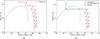 |
Fig. 2 Different pressurisation pathways from 1.5 bar to 151 bar shown in a pressure-enthalpy diagram for CO2, (A) pure compression with inter-cooling with fixed stage pressure ratio, (B) compression to 45 bar followed by cooling/condensation (liquefaction) and final pumping. |
The condensation of the CO2-rich stream is facilitated by a single stage mechanical vapour compression refrigeration cycle named “Refrigeration” in Figure 1. For the refrigeration cycle the key parameters are the isentropic compressor efficiency, the condenser temperature and sub-cooling temperature, the refrigerant evaporator temperature (CO2 condenser) and the super-heating in the evaporator. Different working fluids can be selected, but in the present study only ammonia/R717 is utilised. Alternatively, the liquefaction can be provided by an open or auto-refrigerated cycle using the CO2 itself [13] which may offer benefits, since the external closed-cycle refrigeration can be avoided and less rotating equipment is needed, lowering complexity, maintenance and potentially CAPEX. However, open cycles for CO2 liquefaction seem only to be competitive in terms of levelised cost, when the liquefaction occurs below 15 bar [14], although other factors may be influential such as the level of CO2 impurities, the cooling system used, and the scale of operation. Although the use of open cycles is outside the scope of the current study, future investigations could be relevant.
A variant that still employs refrigeration cooling and pumping is if a pressure Pliq above the critical point, still below the final pressure is specified accompanied by a specified cooling temperature Tliq. Obviously, co-existing vapour and liquid is not possible above the critical point, but the CO2 stream is cooled from the last compression stage into the dense phase region before final pumping to the specified final pressure.
A summary of the key simulation parameters is given in Table 1. Perhaps the most interesting parameters are: the number of compression stages n, and the inclusion of liquefaction at a specified pressure Pliq. Further, the choice of compressor cooling temperature Tin as well as the magnitude of the pressure drop in each compression stage after/inter-cooler are also of particular interest.
Key simulation parameters.
2.2 Thermodynamic model
In order to calculate thermodynamic properties as well as VLE behaviour, an adequate equation of state is required. In the current work CoolProp [15] is used as the main thermodynamic back-end. The option of using REFPROP [16] is also possible in any case calculations are required for mixtures in the two-phase region. Both tools use Helmholtz energy formulations for modelling pure components and mixtures. For pure CO2 the Span-Wagner equation of state is employed [17], for mixtures the method of Lemmon [18] and Kunz [19] is used. For mixtures with CO2 the binary parameters in both CoolProp and REFPROP have been updated with those from EOS-CG [20] and later estimations by Herrig [21].
2.3 Main simulation program
The pressure ratio for each compression stage is assumed to be constant. Thus, for a specified inlet and final outlet pressure of a multi-stage compression process with n stages, the total pressure ratio, Prtot, can be expressed in terms of stage pressure ratio (1)
(1)
The individual stage pressure ratio, Prstage, is![Mathematical equation: $$ {{Pr}}_{\mathrm{stage}}=\sqrt[n]{P{r}_{\mathrm{tot}}}. $$](/articles/stet/full_html/2025/01/stet20240102/stet20240102-eq2.gif) (2)
(2)
In case each compression stage has an associated constant absolute pressure drop, dP, the pressure ratio for each stage needs to be higher, compensating for the built-in pressure drop, in order to achieve the specified total pressure ratio of the multi-stage compression, i.e.,  . For stage i the outlet pressure, Pout,i
, is given as:
. For stage i the outlet pressure, Pout,i
, is given as: (3)with the final pressure, Pout,n
, calculated as
(3)with the final pressure, Pout,n
, calculated as (4)or alternatively as
 (5)
(5)
The above equation is solved for Prstage using the Newton-Raphson method.
For each compressor (and pump) the required power, Wcomp, is calculated by: (6)
(6)
The specific enthalpy at discharge conditions, hdischarge, is the enthalpy change for an ideal isentropic compression process added to the specific enthalpy at suction conditions hsuction. The compressor/pump discharge temperature can be found from a constant pressure/enthalpy process, with enthalpy at discharge are conditions specified as (7)
(7)
The cooling duty, Qcool, for a specific process is modelled as (8)
(8)
Both inlet and outlet specific enthalpies are calculated from known pressures and temperatures. In case there is a pressure drop applied over the cooler, the pressure at outlet conditions is adjusted accordingly. For the economiser, the duty is calculated for a counter-current heat exchanger as the lowest of hot side or cold side pinch, using a pinch temperature of 5 °C. The refrigeration cycle is solved using the CoolProp built-in solver for a simple compression cycle with four cycle states.
The simplified logic and execution flow of the program is visualised in Figure 3. For each calculation step/unit operation considered, i.e., compression, cooling, pumping, the fluid state is recorded both in and out of each operation as well as any required power input (compressor/pump) or heat exchanged (coolers/heat exchangers). The simplest calculation is if no refrigeration/liquefaction/pumping (i.e., via Pliq) is specified as well as if no pressure drop dP in compression stages/coolers is specified and only compression is considered from inlet conditions Pin to the final desired pressure Pcomp = Pfinal. The compression process with n stages is calculated one stage at a time with a fixed pressure ratio Pratio. For each stage i, until the final stage is reached, i.e., i = n, the stage inlet conditions are updated from the previous stage output and each stage is calculated in an iterative way. Liquefaction and pumping is activated if Pliq < Pfinal and Pliq is below the critical pressure of the CO2 stream. The liquefaction temperature, Tliq, is calculated at Pliq and a CO2 vapour fraction (VF) equal to 0. The process includes calculation of the required refrigeration cycle, where the Coefficient of Performance (COP) is the key output that enables scaling of the refrigeration cycle energy/power requirements based on the latent heat of the CO2 condensation. The diagram does not show the complexity of the inclusion of the economiser (heat exchanger) upstream the liquefaction process. In case Pliq is set above the critical pressure, a refrigeration process may still be invoked by specifying a cooling temperature, Tliq, for cooling the supercritical CO2 exiting the last compression stage into the dense liquid region. This is only invoked if the specified Tliq is below the refrigeration cycle condenser temperature, Tcond and below the coolant temperature pinch, Tcool + 10 K.
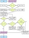 |
Fig. 3 Process simulation logic/program flow chart. |
For all calculations the CoolProp Python wrapper is used. For each state change (cooler, compressor, pump, valve) the properties at the new state are recorded. If using REFPROP as back-end, this is done via the CoolProp wrapper. The CoolProp back-end is applied only for pure CO2. The VLE algorithm in CoolProp does not work well for mixtures (VLE) and in that case REFPROP can be used. REFPROP can be specified to be used for both pure CO2 and mixtures. This work is a continuation of previous works [22, 23] with the purpose of building useful engineering tools on top of high quality open source software packages. The implemented program is developed entirely in Python 3 and also relies on other open source python packages such as pandas [24], matplotlib [25], ht [26], fluids [27], scipy [28] and numpy [29].
2.4 CAPEX estimation method
In this study, the capital cost of equipment is estimated using the methods published by Woods [30]. The equipment cost database by Woods is perhaps the most comprehensive collection available in the public domain [31]. Other comparable database is Peters1 accompanying Peters [32]. The advantage of the Woods database is that specific formulae and scaling relations are provided for each piece of equipment, whereas Peters database is more like a black-box not exposing the underlying cost relations. Alternatively, commercial databases such as Aspen Icarus/Aspen Capital Cost Estimator can be used. Based on internal benchmarks against purchased and installed equipment, the Woods database provides satisfying results.
In Woods [30], the equipment cost in Carbon Steel (CS), CEq,CS, is provided in USD at a reference CEPCI index of 1000. This is also referred to as Free On Board (FOB). For most equipment, a base equipment cost is provided for a reference capacity (flow, weight, power, heat transfer area etc.) with scaling to the actual capacity provided by an equipment (and capacity) specific sizing exponent, n: (9)
(9)
The parameters sourced from Woods [30] relevant for the present study are summarised in Table 2 along with their applicable ranges. The cost relations are commented in the following. In case the upper limit of the applicable range is exceeded for heat exchangers, the required heat transfer area is distributed across several units with the same size, with the individual surface areas summing up to the total required surface area. The heat exchanger costs were estimated based on the overall heat transfer values, U, detailed in Table 3 and a Logarithmic Mean Temperature Difference (LMTD).
Main applied equipment cost relations reported for carbon steel cost in USD and a CEPCI index basis of 1000.
Equipment selection and key assumptions and key sizing parameters applied for cost estimation.
The applicable power, P, (kW) range in Woods [30] for the cost relations for centrifugal compressors was proposed as [2, 4000] and [8000, 25000]. For the purpose of the present study, the two relations were extrapolated up and down, respectively, in order to cover the gap [4000, 8000] by finding the cross-over point between the two relations.
After correcting to an actual CEPCI index of 831.7 (mid Q2 2022), the total installed cost is estimated using the Enhanced Detailed Factor (EDF) method developed by Nils Henrik Eldrup (USN and SINTEF Tel-Tek) and described and applied elsewhere [35, 36]. The EDF method is an equipment factored method and as such a further development of the original Hand method [37]. Compared to other versions of the Hand method, e.g., the method and factors proposed by Woods [30] where installation factors are equipment specific and fixed regardless of equipment size/cost, the EDF installation factors are dependent on the equipment cost instead of type. For the EDF method, the installation factors are high for less expensive equipment and vice versa, lower for more expensive equipment.
The cost estimation using the EDF method is briefly summarised in the following. The total installation factor, FT,CS, is a function of the equipment cost for a single piece of equipment in carbon steel is found in Table 4 for all equipment. Using the installation factors in Table 4, the equipment cost was first corrected to 2020 (using a CEPCI index of 596.2) since the installation factors are on a 2020 basis as described in [38].
For equipment in other materials, a corrected installation factor, FT,other mat., was calculated in accordance with [36]: (10)where, fM is the materials factor cf. Table 5 for accounting for materials other than carbon steel. This applies to the equipment cost and piping costs. A piping installation factor, fpp,CS, relative to equipment cost is also included in Table 4.
The total plant cost, TPC, was then found by summing over all equipment, both CS and other material, multiplying equipment cost with the corresponding installation factor: (11)
(11)
The method described above has been previously implemented and applied by the main author [39] for CAPEX estimation of a biogas upgrading facility including CO2 compression and heat-pumps and for CO2 compression liquefaction via different open and closed liquefaction schemes [14].
2.5 OPEX and levelised cost calculation
For case comparison the total CAPEX is used as one indicator. However, the total CAPEX does not consider annualised costs. Annual costs include several other factors such as fixed operations and maintenance cost (FOPEX), variable operations and maintenance cost (VOPEX) in addition to the annualised CAPEX. A Levelised Cost, for the purpose of this study referred to as Levelised Cost of CO2 Compression, LCOCC, factors this in. Especially the variable cost of electricity required for compression, refrigeration and pumping is an important factor. For example a high CAPEX case with low power requirement may provide a lower LCOCC than a low CAPEX case with high power requirement (depending on the difference in CAPEX and the cost of electricity). In this study we use the following simplified definition of levelised cost in analogy with NREL’s Levelised Cost of Energy (LCOE) [40] which assumes overnight capital cost and O&M costs being invariant over the years2. The LCOCC is given as: (12)
(12)
In Equation (12), CRF is the capital recovery factor; TPC is the overnight capital cost as calculated from Equation (11); O&Mfixed is the yearly fixed Operations and Maintenance cost invariant of the plant load/capacity and O&Mvariable is the yearly Operations and Maintenance cost that scales with plant load. The denominator in Equation (12) is the yearly amount of pressurised CO2, which we set as the nominal mass flow (kg/s) integrated over the year, assuming 100% availability, i.e., 8760 h at the design rate. The variable O&M costs will, for simplicity, be set at the cost of electricity to power compressor, and eventual refrigeration/pumping.
The capital recovery factor is defined as: (13)where i is the interest rate and n is the number of annuities over project lifetime. In this study, the interest is set to 8% (i = 0.08) and the project lifetime is set to 20 years (n = 20). The fixed O&M cost is often expressed as a fraction of the overnight costs. Typical values quoted are in the range 2–6%, depending on the source of information and the process plant type [32, 41, 42]. For sake of simplicity, other fixed costs such as insurance, property taxes, rent of land etc., have not been specifically accounted for; however in the present study O&M costs are fixed to 4%.
3 Results and discussion
3.1 Simulation model validation
The implemented simulation model is tested against a number of references as well as an auto generated case. The first validation is against a simple compression model as implemented in DWSIM 8.5.1. [43] applying the CoolProp property package. Validation and justification of DWSIM is outside the scope of the present study and can be found in, e.g., reference [44]. The validation case is a two-stage compression process compressing 100 kg/s of pure CO2 from 10 to 39 bar with inter-stage cooling to 40 °C and a total pressure drop, dP, of 1 bar. The isentropic efficiency in both compression stages is set to ϵcomp = 0.75. The process is shown in Figure 4 and the results are compared in Table 6.
 |
Fig. 4 Two stage compression process modelled in DWSIM. |
Comparison of simulation results between the current model and DWSIM.
As seen, the results match almost perfectly, which is not a big surprise since the same thermodynamic model is used in both cases and the modelling of compressors and coolers is done in the same way.
The simulation model presented in this study is further bench-marked against a number of literature studies: cases with compression only as well as cases with liquefaction and pumping to the final desired pressure are included. Further, cases considering pressure drop and a single case with significant amounts of impurities are also modelled. The cases have been sourced from literature [8–10]. The case settings and simulation results are summarised in Table 7, including results obtained with the model of the present study. As seen, the simulation model compares well with the literature cases with a maximum deviation of 1.4%, which is considered acceptable also taking into account the different equations of state applied in the modelling.
Simulation model validation against literature data.
3.2 Economic model bench-marking
There is apparently no data available in the open literature and public domain on actual installed costs of CO2 compression systems for high pressure/dense phase pipeline transport, despite a reasonable amount of EOR projects both in the US and Australia making direct comparison between the implemented cost model and real data challenging. Nevertheless, in the following we take a step-wise approach in building confidence in the implemented cost model by first reviewing available data for compressor costs from vendor data, to estimation of full compression system total plant cost and comparison against literature and other software cost models, to finally comparing levelised cost estimates against published studies.
3.2.1 Compressor equipment CAPEX
As part of the EU 7th framework programme project CO2Europipe, OEM budget quotes from Siemens for different CO2 handling capacities ware published [45, 46]. The data pertained to seven-stage integrally geared compressors, compressing CO2 from 1.9 bar to 150 bar [45], with inter-stage cooling applied to 32 °C [45]. Different capacities of 1.5, 3, 6, and 12 MMtonnes/year were considered and quoted. For 1.5 and 3 MMtonnes/year, a single compression train was considered and for 6 and 12 MMtonnes/year 2 and 4 parallel trains were considered, respectively. The compressor cost model applied in the present study, cf. Table 2, is compared to the data from the CO2Europipe project in Figure 5.
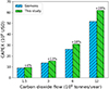 |
Fig. 5 Calculated equipment cost compared to OEM data for compression of CO2 using integrally geared compressors. OEM data is sourced from reference [45]. All cost are on a year 2010 basis (CEPCI = 550.8). Stainless steel has been assumed for compressor casing material. |
As seen in Figure 5 for the lower capacities, the implemented compressor equipment cost model matches OEM data for integrally geared compressors quite well. From 1.5 to 12 MMtonnes/year, the over-prediction of the model increases somewhat, suggesting that the economy of scale built into the model is possibly slightly pessimistic. For the higher flows of 6 and 12 MMtonnes/year, which is simply two and three 3 MMtonnes/year units in parallel, the discrepancy increases even more, suggesting that the OEM has factored in some synergies and discounts when ordering more of the same unit. This is not factored in with the applied cost model.
For inline/barrel type centrifugal compressors, the cost model is compared to an in-house database of installed or quoted equipment costs. The results are shown in Figure 6. Error bars have been added to the calculated values to visualise the ±30% accuracy suggested by Woods [30] for the applied cost relations. As seen from the results, the majority of the compared cases are within the claimed accuracy of the cost relations. However, the data source is sparse, and solid conclusions can not be drawn. Nevertheless, it seems that the model tends to under-predict compressors in the lower driver power range, while the opposite holds for the higher end of the driver power range. While it is often claimed that integrally geared compressors have a lower CAPEX, the data presented in Figures 5 and 6 does not appear to support a general conclusion on this matter. However, a secondary effect is that integrally geared compressors can achieve higher efficiencies. Thus, a lower driver power may be required for an integrally geared compressor compared to an in-line version, resulting in CAPEX savings.
 |
Fig. 6 Calculated cost compared to OEM data for centrifugal in-line/barrel-type natural gas compressors. OEM data is sourced from internal database. All cost are on a year 2010 basis (CEPCI = 550.8). Carbon steel has been applied for compressor casing material. |
3.2.2 Compressor system total plant CAPEX
For the full compression system, a comparison is made against the Integrated Environmental Control Model (IECM) developed for the U.S. Department of Energy’s National Energy Technology Laboratory (DOE/NETL) by Carnegie Mellon University and University of Wyoming [47]. Data has been generated for a four-stage compression of CO2 up to 159 bar with an inter-cooling temperature of 35 °C [48] and a compressor efficiency of 80%. The inlet pressure to the compression system in IECM is not clearly stated, but since it is coupled with MEA-based amine capture, an assumed inlet pressure of 1.5 bar seems reasonable. The IECM model is set up with a maximum compressor duty of 20 MW driver power and so is the model of this study. The comparison between calculations and the IECM model is depicted in Figure 7. From the CAPEX data, the discontinuous nature of the cost models is clearly visible. When the mass flow reaches certain levels, the power surpasses the maximum allowable drive power, and a parallel train is added. This occurs at approximately 60 and 120 kg/s. As seen, the two approaches match remarkably well, with the only exception being the point at 120 kg/s. This is likely due to slight differences in the models, which means the point when the total required power surpasses a multi-plum of 20 MW is a bit off.
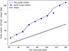 |
Fig. 7 Calculated compression system cost compared to results from IECM. Stainless steel has been assumed. |
Due to lack of CAPEX data for actual constructed CO2 compressor stations, data has been sourced for three natural gas compressor stations: The Egtved compressor station in Denmark, the Wertingen compressor station in Germany and the Everdrup compressor station in Denmark. Key figures for the three compressor stations are summarised in Table 8. The costs for Egtved have been published by the EPC contractors [49, 50], whereas the cost for the Wertingen station is published by the owner/operator [51]. The cost data shown for the Everdrup station is for the FEED design [52]. The EPC tenders have also been published and are approximately 111 and 174 MMUSD (in 2023 value), clearly showing a large spread and also highlighting the large uncertainties in these projects, even when FEED design has been passed. CAPEX calculated within the present study is compared to the available figures in the public domain. The results are shown in Figure 8. The calculated CAPEX is based on a single compression train modelled with the same single compressor duty as shown in Table 8 for each station and then multiplied with the number of parallel trains. As seen, the current model matches quite closely the data for the Egtved and the Everdrup compressor station, whereas there is a significant difference between the calculated and published numbers for the Wertingen compressor station. The reason for the larger difference for this particular case can be difficult to dissect, although one reason may be that costs in addition to the EPC contract have been included, i.e., owners cost, working capital etc. While our model matched FEED/EPC cost estimates quite well, additional cost may be considered to be added to match the total owners cost.
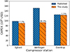 |
Fig. 8 Calculated cost compared to data available for actual constructed compressor stations available in the public domain. |
Total CAPEX for three natural gas compressor stations.
3.2.3 Levelised cost
The present model is compared against published cost estimates (CAPEX) as well as LCOCC. For bench-marking purposes, data is sourced from two references [53, 54]. The first bench-marking is made against data from Hendriks et al. [53]. They presented levelised cost estimates of a four-stage compression process from 1 to 120 bar. They used simple equations for both compression power and total CAPEX. Details about key input are given in Table 9, while calculation output compared to data generated with the simulation program of the present study is summarised in Figure 9. All values of the present study have been adjusted to 2005 costs using a CEPCI index of 444 and an exchange rate from USD to Euro of 0.806 Euro/USD.
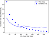 |
Fig. 9 Levelised cost of CO2 compression. Comparison between values calculated in the present study with those of reference [53]. |
As seen in Figure 9, both the data from Hendriks et al. [53] and the data from the present study show a decreasing levelised cost from the lowest to the highest flow. However, there are also noticeable differences. While the data from [53] shows a smooth monotonically decreasing levelised cost as a function of increasing mass flow compressed, the model of the present study is not monotonic. At certain mass flows the levelised cost increases despite an increase in mass flow. This occurs when the cost function adapted in the present study reaches the upper limit of the validity. The implemented compressor cost model has a maximum applicable power of 25 MW. If the required power is higher than this, the mass flow is assumed to be split in two proportionally smaller compressors to avoid exceeding this limit. Due to economics of scale built in to the cost function this results in an increase in cost (smaller units have a higher cost per kW). The cost model in ref. [53] does not have an upper limit of this kind despite the power exceeding 60 MW at the highest CO2 flows. Such a large single unit compressor is not considered realistic, and it gives a good explanation why the present model has higher levelised cost from 70 kg/s and above compared to the model of Hendriks et al. [53]. At mass flows below 60 kg/s, the model of Hendriks et al. shows higher levelised cost than the present study. The main reason for this is the power law exponents used in [53] to account for economy of scale, which is between 0.3 and 0.4 independent on the compressor capacity/power whereas in the present study such exponents are 0.9 at power up to 7000 kW and 0.71 for higher compressor power.
Another study which uses a modified version of the cost function introduced by Hendriks et al. is the study of McCollum and Ogden [54]. They studied CO2 compression from 1 bar up to the critical pressure followed by pumping to a final pressure of 150 bar. Input and calculated output are summarised in Table 10. As seen from the Table 10, the two different approaches compare very well in terms of levelised cost, with the present study predicting slightly higher levelised cost. This minor difference is partly due to the present study predicting slightly higher annualised CAPEX and also slightly higher variable O&M costs. The latter is directly related to the applied cost of electricity and the predicted power requirement. Since the electricity cost is the same, apparently the study of McCollum and Ogden predicts lower power consumption, most likely due to a simplified single equation power model. It is also interesting to note that the variable O&M cost related to power requirement is the dominating factor in the levelised cost (60%), but obviously very sensitive to the choice of electricity cost.
3.3 Carbon capture compression case
The first case studied is a case where only compression is considered from 1.5 to 150 bar, i.e., no liquefaction/pumping. The effect of number of compressor stages is studied in combination with different inter-stage pressure drop being applied to investigate the effect of this parameter, i.e., pressure drop, on the number of compression stages. In this case, a CO2 flow of 100 kg/s is considered and an isentropic compressor efficiency of 80% is applied. Compressor discharge cooling is achieved by means of air-cooled heat exchangers with a discharge temperature of 38 °C and an ambient air temperature of 23 °C. For the techno-economic analysis 20 years lifetime, an interest rate of 8%, an annual fixed OPEX of 4% of total CAPEX, a CF of 1 and an electricity cost of 65 USD/MWh are considered. The CEPCI index is set to 800.6 corresponding to approximately mid 2023. This CEPCI index is used throughout the remaining sections of the present study.
The key indicators, i.e., total compression power, maximum compressor discharge temperature, total CAPEX and LCOCC are investigated as a function of compression stages (1–10) and for different levels of compressor inter-stage pressure drop (due to piping, coolers and scrubbers/coalescers). The simulation results are shown in Figure 10.
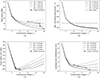 |
Fig. 10 (A) Total power, (B) maximum compressor discharge temperature, (C) total CAPEX, and (D) levelised cost of compression LCOCC as function of number of compression stages and four different levels of inter-stage pressure drop. Compression stage number for minimum power, CAPEX and LCOCC indicated for the different inter-stage pressure drops applied. |
In Figure 10 a number of informative findings appear. As seen from the maximum compression stage temperature (highest of all stages), all cases with four or more stages appear feasible with little effect of the applied inter-stage pressure drop. When zero pressure drop is applied, the minimum power is found at the highest stage number. However, with increasing pressure drop between stages, the optimal number of compression stages decrease. The reason for this is that the cumulative pressure drop for a certain level of stage pressure drop is higher for a higher number of stages. Limiting the number of stages also limits the cumulative pressure drop. Thus, a trade-off appears between a higher number of stages being optimal in terms of compression power and on the other hand a lower number of stages limit the cumulative pressure drop (and hence the power penalty to overcome this pressure drop).
In terms of the total CAPEX the optimum number of stages is four (ignoring the infeasible optima for the highest inter-stage pressure drop due to too high discharge temperature). From this point, and with increasing number of stages, the number of equipment needed increases, i.e., more coolers and more inter-stage scrubbers/coalescers are needed, driving up the CAPEX despite the compression power and hence the CAPEX for the rotating machinery alone decreases. When looking at the aggregate number of LCOCC which factors in both CAPEX and power (via OPEX), it is seen that there is a similar trend as for power: the higher the pressure drop, the less stages are required for minimal LCOCC. It is worth noting that the minimal LCOCC is found at a lower stage number than the minimal power due to the CAPEX generally being optimal at four stages. As an example, the LCOCC optimal number of stages, even with no pressure drop applied, is eight compression stages, even though power minimisation requires more stages.
The results for zero pressure drop is in line with results from Dlamini et al. [10] who also showed that the compression power generally decreased at increasing number of compression stages, although the granularity in terms of number of stages investigated was lower than in the present study.
In the study of Jackson and Brodal [9] the authors investigated the effect of the number of compression stages with a fixed stage pressure drop of 0.5 bar for post-combustion capture and found that nine stages were optimal in terms of power when starting from 1 bar. Adding one more compression stage, i.e., 10 stages in total, resulted in increasing power consumption, likewise for less than nine stages. This is in perfect agreement with the results of the present study for 0.5 bar pressure drop.
It is interesting to note that the results of the present study point to less compressor stages being more optimal when a significant pressure drop between compression stages is accounted for. For the Gorgon injection and storage project [55] inline compressor with fewer inter-cooling stages were selected over an integrally geared compressor with eight compressor stages due to significant pressure drop in inter-coolers and long inter connecting piping (air coolers located away from compressor package) among other things. In that respect the results obtained with the present model seem to support this selection.
3.4 Carbon capture compression/liquefaction/pumping case
3.4.1 Initial case
Following the compression only case for pressurisation of CO2, the concept of compression followed by pumping is introduced and investigated. Below the critical pressure, cooling/liquefaction is required and managed by a refrigerant cycle using ammonia, although use of other refrigerants is possible too. Above the critical pressure, liquefaction as such is not occurring, instead, the CO2 is pumped at the conditions directly after the discharge cooler of the final compression stage. An initial case (case 1) is investigated, which considers the same inputs as the one investigated in the previous section for compression only, in terms of inlet flow, starting and final pressure, and compressor discharge cooler temperature. The main difference is that instead of explicitly defining the number of compression stages, a maximum pressure ratio per stage/section of 2 is applied, which mimics an integrally geared compressor. Further, a fixed pressure drop between compression stages of 0.3 bar is applied. Compression occurs from the initial pressure of 1.5 bar up to the pressure where pumping is initiated (a pressure between 15 and the final pressure of 150 bar). This pressure is referred to as the liquefaction/pumping pressure. The results are shown in Figure 11. In the special case where the pumping pressure equals the final pressure, the case is effectively a compression only case.
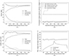 |
Fig. 11 Initial case (case 1). (A) total power requirement as well as subsystem power, (B) Compression pressure ratio and number of compression stages, (C) Total CAPEX as well as subsystem CAPEX, (D) discharge temperature of compressors (max) and liquid CO2 pump, all as a function of pressure where compression ends and pumping is initiated. |
As seen in Figure 11A there is a clear trade-off between the compression and liquefaction (refrigerant compressor) power requirement. At lower liquefaction/pumping pressure, the power demand for liquefaction is high and relatively low for compression, and vice versa at higher liquefaction/pumping pressure. This trade-off is as expected and also in agreement with the findings of Dlamini et al. [10]. Around and just above the critical pressure, there is a peak in the pumping power requirement, which is also seen in the discharge temperature of the pump in Figure 11D. This is due to the relatively high temperature of the compressor discharge temperature of 38 °C (above the critical temperature) leading to a lower density and higher compressibility, sub-optimal for pumping applications. It is interesting to note that the minimum power requirement of 32.7 MW is for the case of compression up to a pressure of 72.5 bar, just below the critical pressure, followed by pumping to the final pressure. For comparison, the power required for the case of compression/liquefaction at 15 bar and compression only is 37.7 and 33.8 MW respectively. Actually, there is a power requirement valley for a range of liquefaction/pumping pressures from approximately 40 bar to the critical pressure where the total power requirement is generally low. Dlamini et al. [10] concluded that a liquefaction pressure of 45 bar leads to a minimisation of the total power, although their analysis did not extend up to the critical pressure only from 15 to 45 bar. Also, the starting pressure (5.7 bara) was different compared to the present study. In their study they also found that a pure compression case with eight stages/sections was slightly more energy-efficient compared to the compression/liquefaction/pumping scenario with three compression stages, which is opposite to the results shown here. One reason may be the lower applied inter-stage pressure drop of 0.1 bar compared to the 0.3 bar applied in this study or that they consider impure CO2.
In Figure 11C the CAPEX of compression and refrigeration displays a similar trade-off as seen from the power in Figure 11A. The pumping power increases from 15 bar up to just above the critical pressure due to decreasing density/increasing compressibility as partly discussed in the previous paragraph. As an end result, the CAPEX is the lowest when the liquefaction/pumping pressure is at its minimum at 15 bar. Then it stays high until after the critical pressure, from where it drops at around 80 bar and then drops until a pure compression case is obtained. The minimum CAPEX is 95.2 MMUSD at a liquefaction pressure of 15 bar and the second lowest CAPEX is for the compression only case with 98.9 MMUSD.
Combining the results in Figure 11 into the levelised cost of compression, LCOCC, as shown in Figure 12, leads to other interesting features. As seen in Figure 12, the minimum levelised cost is not achieved when the CAPEX is lowest nor when power is lowest. It occurs at a liquefaction/pumping pressure of 87 bar. When the power (and hence the variable OPEX) is at its lowest values between 40 bar and the critical pressure, the CAPEX is at its highest values, and when the CAPEX is the lowest (15 bar liquefaction/pumping) the power (variable OPEX) is at its highest. For the selected case, apparently the 87 bar liquefaction/pumping pressure is an optimal compromise between CAPEX and OPEX. It is interesting to note that one of the major compressor OEM’s promote a hybrid solution of combined compression/pumping of CO2 to final delivery, by compression up to 80–83 bar, followed by pumping to the final required pressure [56].
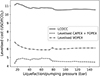 |
Fig. 12 Levelised cost in USD per ton of CO2 for compression/pressurisation for the initial case (case 1) with a break-down into levelised variable OPEX (VOPEX) and CAPEX contribution as levelised CAPEX and levelised fixed OPEX (FOPEX). |
The results quite clearly demonstrates that focusing solely on power or CAPEX when searching for the optimal pressurisation pathway may not identify the best solution minimising the levelised cost of pressurisation. However, it also depends on the project – whether it is CAPEX sensitive or OPEX sensitive, in which case the LCOCC may not be the determining metric. Further, the variance in LCOCC is relatively low, the difference from lowest to highest is 7.3% for the investigated range.
3.4.2 Economy of scale and effect of pressure ratio
In order to check the generality of the above results and conclusions a number of different variation cases are defined.
-
Case 2 As case 1 with reduced mass flow of CO2 of 50 kg/s.
-
Case 3 As case 1 with reduced mass flow of CO2 of 33.3 kg/s.
-
Case 4 As case 1 with reduced mass flow of CO2 of 50 kg/s and the maximum pressure ratio per stage/section increased to four to mimic multi-impeller inline centrifugal compressor(s).
The results of the additional cases including the initial case (case 1), as previously described, are shown in Figure 13 as represented by the calculated levelised cost. Key metrics are extracted from the data and summarised in Table 11. As seen in Figure 13, case 3 to 1 generally display decreasing levelised cost due to higher capacity and hence benefit of economy of scale. The biggest effect is seen from 33.3 kg/s to 50 kg/s. At higher capacities, the effect of economy of scale diminishes due to more compressor units being needed since the maximum single unit capacity is exceeded. In Table 11 it is observed that the lowest CAPEX shifts from liquefaction at 15 bar to pure compression up to 150 bar. The minimum power for case 1–3 is maintained just below the critical pressure, while for the lower capacity cases 2 and 3 the minimum LCOCC is now at a pure compression case, compared to case 1 where pumping from 87 bar was optimal. For case 4, which is calculated at 50 kg/s like case 2, it is interesting to note that, like case 2 (and 3), the minimum CAPEX is obtained for the pure compression case, but the lowest power is obtained at 46.5 bar. The lowest LCOCC is obtained at 96 bar, more in line with case 1. It is also interesting to note that case 4 in some regions leads to lower LCOCC than case 2 when liquefaction/pumping occurs below 60 bar and around 95–100 bar. The reason is the lower number of stages and hence less equipment in terms of coolers and scrubbers/coalescers. Although tempting, we cannot directly conclude that multi-impeller inline centrifugal compressors are better than integrally geared compressors, since the efficiency improvement of the integrally geared compressor has not been taken into account, neither the potentially lower CAPEX.
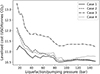 |
Fig. 13 Levelised cost in USD per ton of CO2 for compression/pressurisation for the cases 1 (initial case) to 4. |
Key metrics for case 1–4. For all cases the location in terms of applied liquefaction/pumping pressure for the minimum achieved CAPEX, power and LCOCC, respectively, is listed.
3.4.3 Heat exchanger selection and cooling temperature
To further scrutinize results of the model, additional cases are defined. These additional cases deal with the effect of heat exchanger selection and the applied cooling temperature after compressors (and inter-stage). The basis of the below cases are case 2 from above, i.e., a mass flow of 50 kg/s CO2.
As case 2, but using shell and tube heat exchangers instead of air cooled heat exchangers. This applies to both compressor inter-stage and discharge coolers as well as the refrigerant condenser. The discharge temperature of these coolers are maintained at 38 °C as for case 2.
-
Case 6 As case 5 but with the cooler discharge temperature reduced to 35 °C.
-
Case 7 As case 5 but with the cooler discharge temperature reduced to 30 °C.
-
Case 8 As case 5 but with the cooler discharge temperature reduced to 25 °C.
For all cases, it is assumed that the coolant temperature is 13 °C colder that the cooled CO2. The results of simulating these cases, including case 2 for comparison, are shown in Figure 14. Key metrics for minimum power, CAPEX and LCOCC, respectively, and at which liquefaction/pumping pressure they occur, are compiled in Table 12.
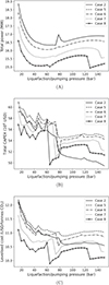 |
Fig. 14 (A) Total power requirement; (B) total CAPEX; (C) levelised cost, all as a function of pressure where compression ends and pumping is initiated for case 2 and case 5–8. |
Starting with power in Figure 14A it is as expected that case 2 and case 5 have identical power requirement. As the discharge temperature is gradually lowered, so is the power requirement. This is also as expected and in agreement with the findings of Dlamini et al. [10] who observe a 4.5% decrease in compression power by reducing coolant temperature by 10 °C. In the present study, a similar decrease in cooling temperature (from case 5 to case 7) results in a 4.3% decrease in power requirements, which is in good agreement. For case 7 and case 8, the power requirement drops significantly at a pumping pressure of approximately 145 bar and 125 bar, respectively. The reason for this drop is that the applied inter-cooler discharge temperature, 30 °C and 25 °C, respectively, actually leads to liquefaction upstream the last compression stage. The corresponding saturation pressures are 72.1 bar and 64.3 bar, respectively. This effectively makes the last compression stage a pumping stage, and in reality, case 7 and 8 have two pumping stages. Due to this “artifact” the power requirement data where this occurs has been omitted from the metrics shown in Table 13. It is also noticed that the spike in power requirement, just above the critical pressure for case 2, is reduced and diminishes when the discharge temperature is reduced below the critical temperature, making the pumping occur in the dense phase region rather than the supercritical region.
Key metrics extracted from Figure 14 for minimum power requirement, minimum CAPEX, and minimum LCOCC and the corresponding liquefaction/pumping pressure at which the minima occur. Data for case 2 (reference for pure CO2), case 9 (post-combustion capture purity), and case 10 (oxy-fuel combustion purity).
When inspecting the CAPEX in Figure 14B the first immediate observation is that switching from air-cooled heat exchangers to shell and tube heat exchangers leads to higher CAPEX. For case 5–8 which employ shell and tube heat exchangers, the CAPEX is generally reduced as the cooler discharge temperature is lowered, which is easily conceived when looking at the corresponding power requirement and correspondingly less cost of compressors and refrigeration systems (also taking into account that the refrigeration loop becomes more effective when the condenser temperature is lowered, i.e., higher COP). The minimum CAPEX for each case generally shifts from a pure compression case (case 2) to a hybrid compression/liquefaction/pumping case and with the minimum CAPEX occurring at gradually lower liquefaction/pumping pressure as the cooler discharge temperature is lowered.
The LCOCC as shown in Figure 14C has some of the same features as just discussed for the CAPEX. Compared to air cooled heat exchangers, the use of Shell and Tube leads to an increase in levelised cost. However, as soon as the discharge temperature is reduced to 35 °C a comparable LCOCC can be achieved. For cases 5–8, the LCOCC generally drops and so does the minimum obtained LCOCC for each case as the discharge temperature is reduced. As seen in Table 12 the location of the minimum LCOCC shifts to lower and lower liquefaction/pumping pressure as the discharge temperature is reduced.
3.4.4 Impurities
In order to study the effect of impurities, two final cases are included both using identical settings as case 2, except for the composition, and with the former requiring REFPROP as thermodynamic back-end:
-
Case 9 Typical composition for post-combustion carbon capture.
-
Case 10 Typical composition for oxy-fuel combustion carbon capture.
The compositions are sourced from Porter et al. [57] is also investigated by Martynov et al. [8] and summarised in Table 14.
Composition of impure CO2 used for calculation of techno-economic parameters. Note: For post-combustion capture trace impurities have been excluded and Argon added to ensure summation of concentrations to 100%.
The results for the two cases (case 9 and 10) with impure CO2 are compared with the reference pure CO2 case (case 2) in Figure 15 with key metrics extracted and summarised in Table 13. As seen in Figure 15, a few immediate observations can be highlighted. The results for pure CO2 and the post-combustion capture composition, which is overwhelming in its CO2 content, generally does not differ much. When a significant amount of impurities is present as for the oxy-fuel case the power consumption is significantly higher, especially when liquefaction/pumping is initiated at lower pressure. The same applies for CAPEX and levelised cost. The lower the pressure from where pumping occurs, the more pronounced the effect. This is mainly due to the effect of a much more challenging liquefaction as also shown in Figure 15D. The saturation temperature drops significantly for a given pressure when the amount of non-condensable gases increase, leading to poor performance of the refrigerant cycle (low COP). With pumping initiated at higher pressure (above approximately 100 bar), the deterioration in power, CAPEX and levelised cost for the oxy-fuel case is moderate compared to the pure CO2 reference and the post-combustion case. When inspecting the key metrics in Table 13, it is again observed that the minimum power required for the oxy-fuel composition is higher than for the pure CO2 and the post-combustion capture case, with the latter being only marginally higher than the pure CO2 case. The minimum CAPEX and LCOCC is similar for all cases, and these key indicators are at the minimum at 150 bar, i.e., for a compression only case. Thus, the optimal architecture of a pressurisation facility will be the same, with main difference being higher power requirement, higher CAPEX and a resulting higher LCOCC as the level of impurities increase.
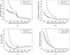 |
Fig. 15 (A) Total CAPEX; (B) levelised cost; (C) total power requirement; (D) refrigeration power requirement, all as a function of pressure where compression ends and pumping is initiated for case 9 and 10 including comparison with case 2. |
The observed increase in power for compression with increasing amounts of impurities is in agreement with the findings of Martynov et al. [8] and was explained by the authors to be mainly related to the corresponding decrease in density of the CO2 mixture as the level of impurities increase, since all the impurities with a significant concentration have a molecular weight lower than that of CO2 (O2, N2 and Ar). Similarly, Martynov et al. also observed an increase-in the refrigeration power required for liquefaction (at 62 bar) as the level of impurities increase in agreement with the results of the present study explained by the widening of the phase envelope and correspondingly lower temperature required for complete liquefaction (lower bubble point temperature).
4 Conclusion
In conclusion, the study presented provides a comprehensive framework for the optimisation and techno-economic analysis of CO2 pressurisation strategies for pipeline transportation. Developed with the use of open-source components and publicly available information, the framework offers significant flexibility to explore various scenario configurations, such as starting and final pressures, inter-stage pressure drop, and cooling temperatures, among others.
The conducted analysis extends beyond solely evaluating work duty reduction, including the assessment of CAPEX, OPEX, and LCOCC. Through this framework, it has been demonstrated that optimal levelised costs do not always correlate with the minimum work, and that for certain scenarios, super-critical and sub-critical pressurisation pathways could provide more cost-effective solutions compared to conventional multi-stage compression.
Bench-marking against existing literature validated the reliability of the simulation results both in terms of the implemented thermodynamic models and equipment and total plant costs models. The study identified that there could be benefits in considering alternative CO2 pressurisation pathways, such as liquefaction and pumping, especially when taking into account a full techno-economic perspective. It is also observed that the optimal pressurisation pathway shifts when certain input parameters are changed.
With the pressing need for effective Carbon Capture, Utilisation, and Storage (CCUS) techniques to mitigate climate change, the findings from this study are timely and relevant. By offering a robust methodology for techno-economic evaluation, this study supports informed decision-making in the CCUS industry, potentially leading to more efficient and economically viable solutions for CO2 handling in pipeline transport systems.
This paper adds value to the body of knowledge on CCUS by combining thermodynamic analysis, process simulation, and economic assessment into a unique and comprehensive framework. It also highlights the importance of open-source tools in facilitating scientific research and allowing for transparency and reproducibility in the presented results.
References
- Andreasen A. (2021) Optimisation of carbon capture from flue gas from a Waste-to-Energy plant using surrogate modelling and global optimisation, Oil Gas Sci. Technol. – Rev. IFP Energies Nouvelles 76, 55. https://doi.org/10.2516/ogst/2021036. [CrossRef] [Google Scholar]
- Wang Q., Zhang D., Li Y., Li C., Tang H. (2024) Numerical simulation study of CO2 storage capacity in deep saline aquifers, Sci. Tech. Energ. Transition 79, 12. https://doi.org/10.2516/stet/2024005. [CrossRef] [Google Scholar]
- Tursunov O., Kustov L., Kustov A. (2017) A brief review of carbon dioxide hydrogenation to methanol over copper and iron based catalysts, Oil Gas Sci. Technol. Rev. – IFP Energies Nouvelles 72, 30. https://doi.org/10.2516/ogst/2017027. [CrossRef] [Google Scholar]
- Wang P.-T., Wu X., Ge G., Wang X., Xu M., Wang F., Zhang Y., Wang H., Zheng Y. (2023) Evaluation of CO2 enhanced oil recovery and CO2 storage potential in oil reservoirs of petroliferous sedimentary basin, China, Sci. Tech. Energ. Transition 78, 3. https://doi.org/10.2516/stet/2022022. [CrossRef] [Google Scholar]
- Eldevik F., Graver B., Torbergsen L.E., Saugerud O.T. (2009) Development of a guideline for safe, reliable and cost efficient transmission of CO2 in pipelines, Energy Procedia 1, 1579–1585. https://doi.org/10.1016/j.egypro.2009.01.207. [CrossRef] [Google Scholar]
- Lu H., Ma X., Huang K., Fu L., Azimi M. (2020) Carbon dioxide transport via pipelines: a systematic review, J. Clean. Prod. 266, 121994. https://doi.org/10.1016/j.jclepro.2020.121994. [CrossRef] [Google Scholar]
- Witkowski A., Majkut M. (2012) The impact of CO2 compression systems on the compressor power required for a pulverized coal-fired power plant in post-combustion carbon dioxide sequestration, Arch. Mech. Eng. 59, 3, 343–360. https://doi.org/10.2478/v10180-012-0018-x. [CrossRef] [MathSciNet] [Google Scholar]
- Martynov S.B., Daud N.K., Mahgerefteh H., Brown S., Porter R.T.J. (2016) Impact of stream impurities on compressor power requirements for CO2 pipeline transportation, Int. J. Greenhouse Gas Control 54, 652–661. https://doi.org/10.1016/j.ijggc.2016.08.010. [CrossRef] [Google Scholar]
- Jackson S., Brodal E. (2019) Optimization of the energy consumption of a carbon capture and sequestration related carbon dioxide compression processes, Energies 12, 9. https://doi.org/10.3390/en12091603. [CrossRef] [Google Scholar]
- Dlamini G.M., Fosbøl P.L., Ness K., Remiezowicz E., Losnegård S.E., von Solms N. (2023) Optimisation of carbon dioxide pressurisation pathways for pipeline offshore delivery, Int. J. Greenhouse Gas Control 128, 103943. https://doi.org/10.1016/j.ijggc.2023.103943. [CrossRef] [Google Scholar]
- Magli F., Spinelli M., Fantini M., Romano M.C., Gatti M. (2022) Techno-economic optimization and off-design analysis of CO2 purification units for cement plants with oxyfuel-based CO2 capture, Int. J. Greenhouse Gas Control 115, 103591. https://doi.org/10.1016/j.ijggc.2022.103591. [CrossRef] [Google Scholar]
- Steimel J. (2020) pyflowsheet, Available at https://github.com/Nukleon84/pyflowsheet. [Google Scholar]
- LE Øi., Eldrup N., Adhikari U., Bentsen M.H., Badalge J.L., Yang S. (2016) Simulation and cost comparison of CO2 liquefaction, Energy Procedia 86, 500–510. The 8th Trondheim Conference on CO2 capture, transport and storage. https://doi.org/10.1016/j.egypro.2016.01.051. [CrossRef] [Google Scholar]
- Cakartas M., Zhou J., Ren J., Andreasen A., Yu H. (2024) Techno-economical evaluation and comparison of various CO2 transportation pathways, Computer Aided Chemical Engineering 53, 2077–2082. https://doi.org/10.1016/B978-0-443-28824-1.50347-1. [CrossRef] [Google Scholar]
- Bell I.H., Wronski J., Quoilin S., Lemort V. (2014) Pure and pseudo-pure fluid thermophysical property evaluation and the open-source thermophysical property library CoolProp, Ind. Eng. Chem. Res. 53, 6, 2498–2508. https://doi.org/10.1021/ie4033999. [CrossRef] [Google Scholar]
- Lemmon E.W., Bell I.H., Huber M.L., McLinden M.O. (2018) NIST Standard Reference Database 23: Reference fluid thermodynamic and transport properties-REFPROP, version 10.0, National Institute of Standards and Technology, Standard Reference Data Program, Gaithersburg. https://doi.org/10.18434/T4/1502528. https://www.nist.gov/srd/refprop. [Google Scholar]
- Span R., Wagner W. (2009) A new equation of state for carbon dioxide covering the fluid region from the triple-point temperature to 1100 K at pressures up to 800 MPa, J. Phys. Chem. Ref. Data 25, 6, 1509. https://doi.org/10.1063/1.555991. [Google Scholar]
- Lemmon E.W., Jacobsen R.T. (1999) A generalized model for the thermodynamic properties of mixtures, Int. J. Thermophys. 20, 3, 825–835. https://doi.org/10.1023/A:1022627001338. [CrossRef] [Google Scholar]
- Kunz O., Wagner W. (2012) The GERG-2008 wide-range equation of state for natural gases and other mixtures: an expansion of GERG-2004, J. Chem. Eng. Data 57, 11, 3032–3091. https://doi.org/10.1021/JE300655B. [CrossRef] [Google Scholar]
- Gernert J., Span R. (2016) EOS-CG: a Helmholtz energy mixture model for humid gases and CCS mixtures, J. Chem. Thermodyn. 93, 274–293. https://doi.org/10.1016/J.JCT.2015.05.015. [CrossRef] [Google Scholar]
- Herrig S. (2018) New Helmholtz-energy equations of state for pure fluids and CCS-relevant mixtures, PhD thesis, Ruhr Universität Bochum, Bochum. [Google Scholar]
- Andreasen A. (2021) HydDown: a Python package for calculation of hydrogen (or other gas) pressure vessel filling and discharge, J. Open Source Softw. 6, 66, 3695. https://doi.org/10.21105/joss.03695. [CrossRef] [Google Scholar]
- Andreasen A., Sousa L.-H., Agustsson G. (2022) An open source tool for calculating CO2 pipeline decompression wave speed, Simulation Notes Europe 32, 4, 187–193. https://doi.org/10.11128/sne.32.tn.10622. [CrossRef] [Google Scholar]
- McKinney W. (2010) Data structures for statistical computing in Python, in: van der Walt S., Millman J. (eds), Proceedings of the 9th Python in Science Conference, Austin, Texas, June 28–July 3, SciPy Proceedings, pp. 51–56. [Google Scholar]
- Hunter J.D. (2007) Matplotlib: a 2D graphics environment, Comput. Sci. Eng. 9, 3, 90–95. https://doi.org/10.1109/MCSE.2007.55. [NASA ADS] [CrossRef] [Google Scholar]
- Bell C. (2023) ht: Heat transfer component of Chemical Engineering Design Library (ChEDL). Available at Available at https://github.com/CalebBell/ht. [Google Scholar]
- Bell C. (2023) fluids: Fluid dynamics component of Chemical Engineering Design Library (ChEDL), Available at https://github.com/CalebBell/fluids. [Google Scholar]
- Virtanen P., Gommers R., Oliphant T.E., Haberland M., Reddy T., Cournapeau D., Burovski E., Peterson P., Weckesser W., Bright J., van der Walt S.J., Brett M., Wilson J., Millman K.J., Mayorov N., Nelson A.R.J., Jones E., Kern R., Larson E., Carey C.J., Polat İ., Feng Y., Moore E.W., VanderPlas J., Laxalde D., Perktold J., Cimrman R., Henriksen I., Quintero E.A., Harris C.R., Archibald A.M., Ribeiro A.H., Pedregosa F., van Mulbregt P., SciPy 1.0 Contributors (2020) SciPy 1.0: fundamental algorithms for scientific computing in Python, Nat. Methods 17, 3, 261–272. https://doi.org/10.1038/s41592-019-0686-2. [NASA ADS] [CrossRef] [Google Scholar]
- Harris C.R., Millman K.J., van der Walt S.J., Gommers R., Virtanen P., Cournapeau D., Wieser E., Taylor J., Berg S., Smith N.J., Kern R., Picus M., Hoyer S., van Kerkwijk M.H., Brett M., Haldane A., Del Río J.F., Wiebe M., Peterson P., Gérard-Marchant P., Sheppard K., Reddy T., Weckesser W., Abbasi H., Gohlke C., Oliphant T.E. (2020) Array programming with NumPy, Nature 585, 7825, 357–362. https://doi.org/10.1038/s41586-020-2649-2. [NASA ADS] [CrossRef] [Google Scholar]
- Woods D.R. (2007) Appendix D: Capital cost guidelines. Rules of thumb in engineering practice, John Wiley & Sons Ltd, Weinheim, Germany, pp. 376–436. ISBN: 9783527611119. https://doi.org/10.1002/9783527611119.app4. [CrossRef] [Google Scholar]
- van Amsterdam M. (2018) Factorial techniques applied in chemical plant cost estimation, PhD thesis, Delft University of Technology, Delft, Netherlands. [Google Scholar]
- Peters M.S., Timmerhaus K.D. (2003) Plant design and economics for chemical engineers, 5th edn, McGraw Hill New Delhi. [Google Scholar]
- Price B. (Ed.), (2012)GPSA engineering data book, 13th edn, Vol. I–II, Gas Processors Suppliers Association, Tulsa, OK. [Google Scholar]
- ASME Boiler and Pressure Vessel Committee. Subcommittee on Pressure Vessels and American Society of Mechanical Engineers (2007) Rules for Construction of Pressure Vessels: Division 1. ASME boiler and pressure vessel code: an international code, American Society of Mechanical Engineers. ISBN: 9780791830680. [Google Scholar]
- Ali H., Eldrup N.H., Normann F., Skagestad R., Øi L.E. (2019) Cost estimation of CO2 absorption plants for CO2 mitigation – method and assumptions, Int. J. Greenhouse Gas Control 88, 10–23. https://doi.org/10.1016/j.ijggc.2019.05.028. [CrossRef] [Google Scholar]
- Aromada S.A., Eldrup N.H., Øi L.E. (2021) Capital cost estimation of CO2 capture plant using enhanced detailed factor (EDF) method: installation factors and plant construction characteristic factors, Int. J. Greenhouse Gas Control 110, 103394. https://doi.org/10.1016/j.ijggc.2021.103394. [CrossRef] [Google Scholar]
- Hand W. (1958) From flow sheet to cost estimate, Pet. Ref. 37, 331–337. [Google Scholar]
- Shirdel S., Valand S., Fazli F., Winther-Sørensen B., Aromada S.A., Karunarathne S., Øi L.E. (2022) Sensitivity analysis and cost estimation of a CO2 capture plant in aspen HYSYS, ChemEngineering 6, 2. https://doi.org/10.3390/chemengineering6020028. [CrossRef] [Google Scholar]
- Jensen E.H., Andreasen A., Jørsboe J.K., Andersen M.P., Hostrup M., Elmegaard B., Riber C., Fosbøl P.L. (2024) Electrification of amine-based CO2 capture utilizing heat pumps, Carbon Capture Sci. Technol. 10, 100154. https://doi.org/10.1016/j.ccst.2023.100154. [CrossRef] [Google Scholar]
- Short W., Packey D.J., Holt T. (1995) A manual for the economic evaluation of energy efficiency and renewable energy technologies, Technical Report NREL/TP-462-5173, National Renewable Energy Laboratory, Golden, CO, https://www.nrel.gov/docs/legosti/old/5173.pdf. [Google Scholar]
- Towler G., Sinnott R. (2013) Chemical engineering design, 2nd edn, Butterworth-Heinemann, Boston, MA. ISBN: 978-0-08-096659-5. https://doi.org/10.1016/B978-0-08-096659-5.00001-8. [Google Scholar]
- Seider W.D., Lewin D.R., Seader J.D., Widagdo S., Gani R., Ng K.M. (2016) Product and process design principles: synthesis, analysis and evaluation, Wiley, New York, NY. [Google Scholar]
- De Medeiros D.W.O. (2023) DWSIM – the open source process simulator. Available at https://dwsim.org/. [Google Scholar]
- Andreasen A. (2022) Evaluation of an open-source chemical process simulator using a plant-wide oil and gas separation plant flowsheet model as basis, Period. Polytech. Chem. Eng 66, 3, 503–511. https://doi.org/10.3311/PPch.19678. [CrossRef] [Google Scholar]
- Mikunda T., van Deurzen J., Seebregts A., Tetteroo M., Kersemakers K., Apeland S., CO2Europipe (2011) Towards a transport infrastructure for large-scale CCS in Europe, D3.3.1 Legal, financial and organizational aspects of CO2 pipeline infrastructures, Technical Report, EU CO2Europipe Consortium, TNO, Utrecht, The Netherlands. [Google Scholar]
- Mallon W., Buit L., van Wingerden J., Lemmens H., Eldrup N.H. (2013) Costs of CO2 transportation infrastructures, Energy Procedia 37, GHGT-11 Proceedings of the 11th International Conference on Greenhouse Gas Control Technologies, 18–22 November 2012, Kyoto, Japan, 2969–2980. https://doi.org/10.1016/j.egypro.2013.06.183. [CrossRef] [Google Scholar]
- Integrated Environmental Control Model (IECM) (2023) A tool for calculating the performance, emissions, and cost of a fossil-fuelled power plant. Available at https://www.uwyo.edu/iecm/index.html. [Google Scholar]
- IECM Technical Documentation (2018) Amine-based post-combustion CO2 capture. Available at https://www.uwyo.edu/iecm/bfiles/documentation/201901iecmtdamine-based-co2-cap.pdf. [Google Scholar]
- Aarsleff (2023) Kompressor station ved Egtved. Available at https://www.aarsleff.dk/img/5932/0/0/Download/160-kompressorstation-ved-egtved-dk. [Google Scholar]
- Streicher (2023) Compressor station Egtved. Available at https://www.streicher.de/fileadmin/userupload/www.streicher.de/Referenzen/Rohrleitungs–Anlagenbau/EPC-Bereich/ProjektberichtEgtvedDaenemarkENrev2red.pdf. [Google Scholar]
- Bayernets (2023) Wertingen compressor station in figures. Available at https://www.bayernets.de/fileadmin/Dokumente/Pressemitteilungen/2019-12-17/EN/FactsheetWertingenCompressorStation.pdf. [Google Scholar]
- The Danish Complaints Board for Public Procurement (2020) Verdict: MMEC Mannesmann Gmbh vs. Energinet Gas TSO A/S J.nr.: 20/04052. Available at https://kammeradvokaten.dk/media/7967/mmecmannesmanngmbhmodenerginetgastsoas.pdf. [Google Scholar]
- Hendriks C., Graus W., van Bergen F. (2004) Global carbon dioxide storage potential and costs, Technical Report EEP-02001, ECOFYS/TNONITG, Rijksinstituut voor Volksgezondheid en Milieu, The Netherlands. [Google Scholar]
- McCollum D.L., Ogden J.M. (2006) Techno-economic models for carbon dioxide compression, transport, and storage and correlations for estimating carbon dioxide density and viscosity, Technical Report UCD-ITS-RR-06-14, Institute of Transportation Studies, University of California, Davis, CA. Available at https://itspubs.ucdavis.edu/downloadpdf.php?id=1047. [Google Scholar]
- Musardo A., Pelella M., Patel V., Weatherwax M., Giovani G., Cipriani S. (2013) CO2 compression at world’s largest carbon dioxide injection project, in: Proceedings of the Second Middle East Turbomachinery Symposium, Doha, Qatar, 17–20 March. [Google Scholar]
- Brun K., Pettinato B., Ross S., Omatick T., Thorp J. (2023) CO2 compression challenges, World Pipelines, 23. [Google Scholar]
- Porter R.T., Fairweather M., Pourkashanian M., Woolley R.M. (2015) The range and level of impurities in CO2 streams from different carbon capture sources, Int. J. Greenhouse Gas Control 36, 161–174. https://doi.org/10.1016/j.ijggc.2015.02.016. [CrossRef] [Google Scholar]
All Tables
Main applied equipment cost relations reported for carbon steel cost in USD and a CEPCI index basis of 1000.
Equipment selection and key assumptions and key sizing parameters applied for cost estimation.
Key metrics for case 1–4. For all cases the location in terms of applied liquefaction/pumping pressure for the minimum achieved CAPEX, power and LCOCC, respectively, is listed.
Key metrics extracted from Figure 14 for minimum power requirement, minimum CAPEX, and minimum LCOCC and the corresponding liquefaction/pumping pressure at which the minima occur. Data for case 2 (reference for pure CO2), case 9 (post-combustion capture purity), and case 10 (oxy-fuel combustion purity).
Composition of impure CO2 used for calculation of techno-economic parameters. Note: For post-combustion capture trace impurities have been excluded and Argon added to ensure summation of concentrations to 100%.
All Figures
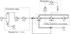 |
Fig. 1 General CO2 pressurisation cycle. The flowsheet is generated using pyflowsheet [12]. |
| In the text | |
|
Fig. 2 Different pressurisation pathways from 1.5 bar to 151 bar shown in a pressure-enthalpy diagram for CO2, (A) pure compression with inter-cooling with fixed stage pressure ratio, (B) compression to 45 bar followed by cooling/condensation (liquefaction) and final pumping. |
| In the text | |
|
Fig. 3 Process simulation logic/program flow chart. |
| In the text | |
|
Fig. 4 Two stage compression process modelled in DWSIM. |
| In the text | |
|
Fig. 5 Calculated equipment cost compared to OEM data for compression of CO2 using integrally geared compressors. OEM data is sourced from reference [45]. All cost are on a year 2010 basis (CEPCI = 550.8). Stainless steel has been assumed for compressor casing material. |
| In the text | |
|
Fig. 6 Calculated cost compared to OEM data for centrifugal in-line/barrel-type natural gas compressors. OEM data is sourced from internal database. All cost are on a year 2010 basis (CEPCI = 550.8). Carbon steel has been applied for compressor casing material. |
| In the text | |
|
Fig. 7 Calculated compression system cost compared to results from IECM. Stainless steel has been assumed. |
| In the text | |
|
Fig. 8 Calculated cost compared to data available for actual constructed compressor stations available in the public domain. |
| In the text | |
|
Fig. 9 Levelised cost of CO2 compression. Comparison between values calculated in the present study with those of reference [53]. |
| In the text | |
|
Fig. 10 (A) Total power, (B) maximum compressor discharge temperature, (C) total CAPEX, and (D) levelised cost of compression LCOCC as function of number of compression stages and four different levels of inter-stage pressure drop. Compression stage number for minimum power, CAPEX and LCOCC indicated for the different inter-stage pressure drops applied. |
| In the text | |
|
Fig. 11 Initial case (case 1). (A) total power requirement as well as subsystem power, (B) Compression pressure ratio and number of compression stages, (C) Total CAPEX as well as subsystem CAPEX, (D) discharge temperature of compressors (max) and liquid CO2 pump, all as a function of pressure where compression ends and pumping is initiated. |
| In the text | |
|
Fig. 12 Levelised cost in USD per ton of CO2 for compression/pressurisation for the initial case (case 1) with a break-down into levelised variable OPEX (VOPEX) and CAPEX contribution as levelised CAPEX and levelised fixed OPEX (FOPEX). |
| In the text | |
|
Fig. 13 Levelised cost in USD per ton of CO2 for compression/pressurisation for the cases 1 (initial case) to 4. |
| In the text | |
|
Fig. 14 (A) Total power requirement; (B) total CAPEX; (C) levelised cost, all as a function of pressure where compression ends and pumping is initiated for case 2 and case 5–8. |
| In the text | |
|
Fig. 15 (A) Total CAPEX; (B) levelised cost; (C) total power requirement; (D) refrigeration power requirement, all as a function of pressure where compression ends and pumping is initiated for case 9 and 10 including comparison with case 2. |
| In the text | |
Current usage metrics show cumulative count of Article Views (full-text article views including HTML views, PDF and ePub downloads, according to the available data) and Abstracts Views on Vision4Press platform.
Data correspond to usage on the plateform after 2015. The current usage metrics is available 48-96 hours after online publication and is updated daily on week days.
Initial download of the metrics may take a while.