")
")
| Issue |
Sci. Tech. Energ. Transition
Volume 81, 2026
|
|
|---|---|---|
| Article Number | 4 | |
| Number of page(s) | 16 | |
| DOI | https://doi.org/10.2516/stet/2026001 | |
| Published online | 24 March 2026 | |
Regular Article
Assessment of the voltage stability of the power system using stability indices and artificial neural network
1
Department of Electrical Engineering, Government Engineering College, Siwan, Bihar 841226, India
2
Department of Electrical Engineering, National Institute of Technology, Patna, Bihar 800005, India
3
Department of Electrical Engineering, Rajkiya Engineering College, Ambedkar Nagar 224122, UP, India
4
Department of Electrical Engineering, Rajkiya Engineering College, Mainpuri 205001, Uttar Pradesh, India
5
Department of Electrical and Electronics Engineering, Nalanda College of Engineering, Chandi, Nalanda 803108, Bihar, India
6
Department of Mechanical Engineering, Government Engineering College, Siwan, Bihar 841226, India
7
Assistant Professor (EE), Department of Science, Technology and Technical Education, Govt. of Bihar, Patna, Bihar 800013, India
* Corresponding author: This email address is being protected from spambots. You need JavaScript enabled to view it.
Received:
30
September
2024
Accepted:
26
January
2026
Abstract
Voltage Stability Indicators (VSI) play a significant role in determining the voltage stability of the power system. In order to forecast the voltage instability of the system using voltage stability indicators, this paper presents an implementation of an Artificial Neural Network (ANN) based on the Levenberg–Marquardt (LM) technique. In this context, the performance of three voltage stability indicators – the Line Voltage Stability Index (LVSI), the Line stability index (Lmn), and the Fast Voltage Stability Indicator (FVSI) are compared. Based on the maximum active power loadability of load buses of the IEEE 14-bus and IEEE 118-bus systems, these indicators are used to assess their vulnerability. The LVSI, Lmn, and FVSI indices obtained from the Newton-Raphson method of the most severe buses of both test systems are compared with the forecasted values by the ANN method under base load to critical loading conditions. The real and reactive power losses of the lines associated with the most severe bus of the systems and totally real and reactive power losses of the systems are forecasted by the MATLAB NN toolbox under wide variations in active power loading. The Static Synchronous Compensator (STATCOM) is used to enhance the voltage of the most severe bus of the system. The outcomes show that the methods for assessing voltage stability using ANN under the variation of the real power demand of the critical bus is highly précised and technically feasible.
Key words: ANN / Collapse / FACTS / Line indices / Voltage stability
© The Author(s), published by EDP Sciences, 2026
 This is an Open Access article distributed under the terms of the Creative Commons Attribution License (https://creativecommons.org/licenses/by/4.0), which permits unrestricted use, distribution, and reproduction in any medium, provided the original work is properly cited.
1 Introduction
Voltage instability arises as a result of a system’s condition varying fortuitously due to a rapid increase in load demand. Additionally, the current power system is used extremely close to its stability thresholds. The unexpected growth in the electricity system’s load demand restructuring lowers the overall system’s efficiency and dependability [1]. Voltage drops, power outages, and the conflict between transmission and generation result in an unsteady and vulnerable system. A few literary analyses demonstrate that the development of physical ideas and mathematical representations of voltage constancy has advanced steadily. They either depend on the viability of solutions for load flow, such as P-V and Q-V curves, quick load disconnected flow, Continuous Power Flow (CPF) [2, 3], or on other methods, such as modal analysis [4], best voltage security analysis, power transfer, singularity, or traffic control. The numerous operating variables of the system under varied conditions affect the node’s susceptibility. Any single variable might not be sufficient to determine voltage stability at a given network node. To prevent any serious systemic problems, the interdependence of these variables must be discussed in all courses. Voltage stability indices (VSIs) are derived in order to identify voltage stability margins, maximum load, weak lines, and weak bus in the network. VSIs are defined for a line or bus and are classified based on considerations, critical values, regional or universal stability investigation, and network modeling [5]. Sensitivity is examined in some articles by estimating the system’s eigenvalues or using a proximity indicator [6]. The system variable quantity (Jacobian matrix) is the major criterion used to categorize these indices. The required information can be gathered from PMUs or static evaluation, and both offline and online modes can be applied. Voltage collapse point characteristics serve as the foundation for all VSIs [4]. Due to its limited nature, voltage collapse happens when the reactive power demand cannot be satisfied. Devices called FACTS keep the reactive power supply dynamic [7, 8]. They are employed in the regulation of voltage, load sharing between parallel corridors, management of loop flows, and power flow. Recently, Artificial Neural Networks (ANN), which are ideal for a large power system, have been on the scene to function more rapidly and decisively. It may result in a strong reliance between the input and the output. It can be used for security, load forecasting, tracking transient stability assessment, the flexibility of protective systems, and many other things [9, 10].
It has already been discussed how to assess voltage stability using a variety of indicators [1, 5, 11]. Several artificial intelligence paradigms have been linked with a voltage instability indicator in the past Devaraj and Roselyn [12], Subramani et al. [13] proposed the Radial Base Function Neural Network (RBFNN) and Cascade Based Feed Forward Neural Network (CBFNN) approaches utilizing the Global Voltage Stability Indicator (GVSI), while Borazjani et al. trained the data using the Linear Programming (LP) methodology technique [6]. A Jacobian matrix calculation is necessary for GVSI. The voltage collapse point and the voltage stability margin are calculated using VSIs based on the Jacobian matrix [5]. In contrast to the parametric voltage stability indicators, it requires more computation time and becomes more difficult with any topological alteration or system size. Therefore, parametric VSIs are preferable for the examination of the stability. Devaraj and Roselyn used RBFNN with reduced input topographies and L index in a NN for online assessment [12], which allowed for high accuracy and rapid calculations. Goh et al.’s definition of line indicators [14] used all of the indicator’s parametric parameters as input to create VSIs.
Three-line indices were compared with Newton-Raphson and ANN approaches for the forecast of the voltage stability of the electrical network [15]. The voltage stability margin was investigated using an ANN [16]. In [17], the study suggested a PMU measurement-based method for observing and evaluating the voltage stability margin that uses an ANN hybrid model. The meta-parameter of ANNs is optimized by Particle Swarm Optimization (PSO) to increase the rate of convergence. The article [18] suggests an Artificial Neural Network (ANN) based method for online maintenance control of the grid-equipped Voltage Source Converters (VSCs) with the pole-tracking feature to address the stability problem of weedy grid-equipped VSCs. In the study [19], a method for very short-term grid frequency and voltage forecast was developed using Deep Recurrent Neural Networks (DRNN) and ANNs. To lower the computational charge of the traditional Power Flow (PF) method, [20] introduces a brand-new planning tool for Hopfield Neural Networks (h-HNN) based on heuristics. The suggested strategy is an energy function-based, Jacobian-free strategy that was developed using the system’s power residuals. [21] focuses on giving a thorough overview of the most recent Machine Learning (ML) methods used for online voltage stability assessment. A novel unified voltage collapse proximity indicator based on intelligent control and generalized approximate reasoning was proposed in [22] as a method for determining the voltage of the system’s weak buses. In order to rank the load buses and determine which is the most crucial, [23] proposed a novel method for determining each load bus’s maximum loading limit using a modified continuous power flow method. A controller was proposed in [24] that can lower the system parameter peak values and uncertainties that are increased during grid faults. The transient stability assessment methods using Deep Reinforcement Learning (DRL) and Reinforcement Learning (RL) are also briefly discussed in [25]. The primary reason for voltage collapse is a deficiency in the production and support of reactive power. Rearranging the schedule for the generation of reactive power or adding more reactive support to the system can meet the reactive power demand [26]. In the [27] study, contingencies are first ranked according to their voltage stability margin, and then the most crucial line of the IEEE 14-bus system is identified using the line stability factor (Lqp), Fast Voltage Stability Index (FVSI), and the Line stability index (Lmn) methods. The Lmn [28], FVSI [29], Lqp [30], and Line Voltage Stability Index (LVSI) [31] were investigated to assess the severity of lines.
In this study, the LVSI, Lmn, and the FVSI are compared for their performance to assess the voltage stability of the system. These indicators are used to determine how vulnerable the IEEE 14-bus and IEEE 118-bus systems are based on the maximum active power loadability of their load buses. The LVSI, Lmn, and FVSI indices were computed for the most severe buses of both test systems using the Newton-Raphson approach and are compared with the values predicted by the ANN method under base load to critical loading circumstances. The NN methodology could be valuable for a big electrical network if the NN configuration is not overly complex, because the findings would be quicker with better accuracy, which is the most difficult condition for voltage stability analysis. So, since this research talks about reducing the number of dimensions, the simple, quick, and accurate NN method using the voltage stability indices is used here to predict the bus voltage stability using only some of the input variables for training. The Static Synchronous Compensator (STATCOM) is also employed to raise the voltage stability of the system’s most critical bus.
2 Voltage Stability Indices (VSI)
Both the system’s static and dynamic elements have been covered by VSI. This method, which provides the precise dynamics of the voltage stability, is an approximation of the dynamic modeling of the two bus systems. The weakest bus, line, maximum allowable loadability, and distance to the voltage collapse point can all be found using the line indicators. There are already numerous line indications discussed in a variety of literary works. In this context, a successful application is shown together with a performance comparison of three indicators, namely the line stability factor (LQP), the Fast Voltage Stability Indicator (FVSI), and the Line Voltage Stability Index (LVSI). How VSIs are used to figure out the maximum load that can be put on the system before the voltage becomes unstable is discussed below.
2.1 Fast Voltage Stability Indicator (FVSI)
The authors in [29] proposed a fast voltage stability index (FVSI). This index is a simplification of a previously produced voltage stability index that was connected to a line at the transmitting end of a two-bus system representation. The performance of the suggested indication was evaluated using the IEEE 30-Bus reliability test system using the devised index. As a result, equation (1) can be used to define the equation for the FVSI index. (1)
(1)
where V is the voltage at the sending end, X is the line reactance, and Z is the line impedance. Q is the reactive power at the receiving end. An instability point is going to be reached when the line voltage stability indexes show an FVSI that is very near to unity (1.0).
2.2 Line Stability Index (Lmn)
In [28], the properties of the line stability factors were described. Mathematically is represented as: (2)
(2)
Where δ is the power angle for the line connected from the ith bus to the jth bus. For a system to operate reliably and securely, its Lmn value needs to be lower than 1.
2.3 Line Voltage Stability Index (LVSI)
This index was proposed in [31], which takes into account line charging capacitances and resistances, which are typically ignored by many voltage stability indices, because it is based on transmission line properties. For the suggested index to determine the voltage stability condition of various lines, only bus voltage phasor data is needed. The value of the index ranges from 2 to 1. While a score close to 1 indicates a poor state of voltage stability, a value close to 2 indicates a steady state of voltage. The application results further demonstrate the capability of the index LVSI to recognize voltage breakdown points and critical lines. Using the suggested index, the voltage stability state of various lines can be evaluated. The following equation represents the LVSI index. (3)
(3)
where, A is part of the ABCD parameter of the line, α is the angle A parameter, and β is the angle of the B parameter.
3 Static Synchronous Compensator (STATCOM)
In order to control the reactive power flow over a power network and consequently improve the stability of the power network, a power electronic device called a STATCOM, or static synchronous compensator, uses force-commutated devices like IGBT, GTO, etc. Since STATCOM is a shunt device, it is shunt-connected to the line. Static Synchronous Condenser (STATCON) and Static Synchronous Compensator (STATCOM) are both names for the same device. It belongs to the FACTS family of devices, which stands for Flexible AC Transmission System. Synchronous in STATCOM refers to the ability to generate or absorb reactive power in synchrony with the need to maintain the power network’s voltage.
A STATCOM can be utilized for a wide range of applications since it is a quick, multi-quadrant source of reactive power, and dynamic, but it is best suited for maintaining the grid during fault, transient, or contingency events. Placing a STATCOM along a transmission line to enhance system power flow is one common application. The STATCOM won’t do much when things are running normally, but if a neighboring line fails, the previously provided power is compelled onto other transmission lines. Normal power flow causes a voltage drop rise as a result, but if a STATCOM is available, it can give reactive power to raise the voltage until the fault is fixed (if temporary) or till an existing capacitor can be turned in (if fixed). In some circumstances, a STATCOM can be placed at a switchgear to help support more than one line instead of just one, and to help simplify protection on the line that has a STATCOM on it. The STATCOM can bidirectionally exchange reactive power and is always connected in a shunt. This device’s main applications are dynamic (rapid) correction, voltage support, oscillation damping alleviation, and enhancing the transient stability limit. The Magnetic Circuit (MC), Voltage Source Converter (VSC), shunt breaker, shunt coupled transformer, and protection and control unit of STATCOM are all depicted in Figure 1.
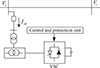 |
Figure 1 A schematic illustration of STATCOM using two bus systems. |
4 Artificial Neural Network (ANN)
The functioning pattern of biological human brains served as the basis for the neural network, a computational technique. Input, hidden, and output layers are all combined to form the neural network. Depending on the problem, a further hidden layer may have multiple layers. Different nodes connected by node connections that have bias values and specific weights are used to connect all three layers. Prediction networks come in a variety of forms, but the problem determines which network will produce the best results. Networks with multiple layers are widely used and produce the desired accuracy in a particular sense, as shown in Figure 2. Feed-forward backpropagation is the most popular network for problem prediction in electrical engineering.
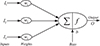 |
Figure 2 ANN network. |
The output of the ANN network given in Figure 2 is written as: (4)where input variables, weights, bias, and output are represented by I, w, b, and O, respectively. Here, a Back Propagation Neural Network (BPNN) is employed, equipped with sigmoid hidden neurons and linear output neurons. This makes the system more nonlinear for the vanishing gradient problem. The Newton algorithm’s training speed and Error Back Propagation (EBP) stability are interpolated by the LM algorithm. This algorithm typically uses more memory but takes less time. Optimized weights are used to reduce error. The weight initialization, feedforward, spread back error, and weights and biases update phases make up the backpropagation training algorithm. The magnitude and frequency of the system voltage can be represented as non-linear functions of real power and reactive power for the static load model. Since voltage transients decay more quickly, voltage stability is given priority over frequency. The input and output can be written as:
 (5)
(5)
The input of the hth hidden layer, (6)
(6)
The output of the hth hidden layer, (7)
(7)
Input if Oth hidden layer, (8)
(8)
The output of the Oth hidden layer, (9)
(9)
Weight updating in between ith and hth layers, (10)
(10)
Weight updating in between hth and Oth layers, (11)
(11)
For the new iteration, weight updating, (12)where, is the learning rate.
5 Results and discussion
IEEE 14-bus and IEEE 118-bus systems have been used to examine the applicability of the proposed method. The simulation is being carried out by a computer program that has been created in the MATLAB environment. For the largest absolute bus power mismatch, a convergence tolerance of p.u. has been selected. Studies based on the loading combination have been conducted in each test system for various criteria. Testing all of the load buses under base case conditions, as well as with heavy active loading at various nodes, identifies the performance of the overall system.
The weakest bus in the system is the bus that has the lowest bus voltage under critical active loading conditions. The LVSI, Lmn, and FVSI indices value for a particular node is the average value of the line indices of lines associated with that node. The LVSI, Lmn, and FVSI indices for the critical bus of the system evaluated from the Newton-Raphson method are compared with forecasted ANN values. The real and reactive power losses of the systems are also predicted by the ANN method. The pictorial representation of the proposed approach is shown by the flow chart in Figure 3.
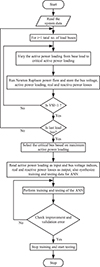 |
Figure 3 Flow chart of the proposed approach. |
5.1 Heavy active power loading at each bus
5.1.1 IEEE 14-bus system
To investigate the maximum active power loading of each bus of the system, the active power loading on each bus increases from the base load until the divergence of the load flow solution. The maximum active power loadability of a bus is the maximum loading after which the solution of load flow will diverge. For the IEEE 14-bus system, bus number 4 has the highest maximum active power loadability of 7.002 p.u. whereas bus number 14 has the lowest maximum active power loadability, 1.62 among the maximum active power loadability of all load buses p.u.as shown in Table 1. So, bus number 14 is considered the most severe bus of the system, which was also found in [32]. So, this bus can be chosen as the most appropriate place for placing the reactive power support devices like Static Var Compensator (SVC) and STATCOM. For this bus, the line indices LVSI, Lmn, and FVSI values are obtained as 1.00051, 0.99411, and 0.99395, respectively, which are very close to their boundary limits (2 for LVSI, 1 for Lmn, and FVSI). Figure 4a shows that the line indices LVSI, Lmn, and FVSI values approach unity as active power loading increases from base load to maximum permissible load at bus number 14. Whereas Figure 4b shows the bus voltage magnitude of the bus versus the active power loading curve with and without deployment of the STATCOM at bus number 14. During heavy active loading conditions, the STATCOM improves the voltage profile and enhances the active power loading capability of the most severe buses.
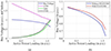 |
Figure 4 (a) Line indices LVSI, Lmn, FVSI, and bus voltage magnitude of bus 14 vs active power loading at bus 14. (b) Bus voltage magnitude of bus 14 with and without STATCOM under heavy active power loading at bus 14. |
Line indices values of load buses of IEEE 14-bus under the critical active power loading.
5.1.2 IEEE 118-bus system
The active power loading on each bus increases from base load to peak load. The critical active power loading on 10 load buses (out of 89 load buses) is depicted in Table 2. It is observed that among all 89 load buses, bus number 44 has the lowest maximum active power loading capability, i.e., 2.87 p.u. At maximum permissible active power loading, the bus voltage magnitude of bus number 44 is 0.63282 p.u. Whereas bus number 11 has the highest active power loading capability, i.e., 12.36 p.u. The LVSI, Lmn, and FVSI indices of load buses during critical active power loading conditions are also depicted in Table 2. Bus number 44 is decided as the most critical bus of the IEEE 118-bus system, at which shunt FACTS devices can be connected to enhance the active power loading capability and bus voltage magnitude of this bus.
Line indices values of load buses of IEEE 118-bus under the critical active power loading.
From Figure 5a, it is observed that as the active power loading on the most severe bus 44 increases, the Lmn and LVSI indices increase from zero to unity. In this situation, the value of LVSI also decreases from 2 to its critical value (unity). After deploying the STATCOM at bus number 44, the bus voltage profile of bus 44 is improved as shown in Figure 5b.
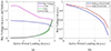 |
Figure 5 (a) Line indices LVSI, Lmn, FVSI, and bus voltage magnitude of bus 44 vs active power loading at bus 44. (b) Bus voltage magnitude of bus 44 with and without STATCOM under heavy active power loading at bus 44. |
5.2 Real and reactive power losses during heavy active power loading at critical bus
5.2.1 IEEE 14-bus system
Lines (14-13) and (14-9) are associated with the most severe bus of the system. So, these lines are highly prone to voltage instability. As the active power loading increases on bus 14, the real and reactive power losses of the lines (14-13) and (14-9) are increased. The rate of increase in the real and reactive power losses of line (14-9) is higher than that of line (14-13). So, the line (14-9) is highly sensitive towards voltage stability with increments in active power loading, as shown in Figure 6. In a similar manner, the total reactive power loss of the IEEE 14-bus system increases with high rate than real power loss on increasing the active power loading at bus 14 as shown in Figure 7.
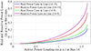 |
Figure 6 Real and reactive power losses of the lines (14-13) and (14-9). |
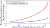 |
Figure 7 Total real and reactive power losses of the IEEE 14-bus system. |
5.2.2 IEEE 118-bus system
The real and reactive power losses of the lines associated with the most severe bus 44 have been measured by Newton-Raphson’s load flow under wide variations in the load of bus 44. The rate of increase of reactive power losses is more than the rate of growth of real power losses as the active power loading increases from base load to peak load, as shown in Figure 8. The reactive power loss of the (44-45) is maximum at critical active loading at bus 44. Whereas, for the line (44-43) at active power loading near base load, the real power loss is more than the reactive power loss, but after a certain active power loading, the reactive power becomes more than the real power loss. Similarly, on increasing the active power loading at bus 44, the real and reactive power losses of the system increase. And the rate of increment of reactive power loss of the system is higher than real power loss, as shown in Figure 9.
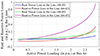 |
Figure 8 Real and reactive power losses of the lines (44-43) and (44-45). |
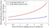 |
Figure 9 Total real and reactive power losses of the IEEE 118-bus system. |
5.3 Assessment of voltage stability using ANN
5.3.1 IEEE 14-bus system
By increasing the active power load of the critical load bus, the NR static load flow analysis is used to calculate the LVSI, Lmn, and FVSI indices values. The severity of the bus is indicated by these values. The amount of maximum load that can be injected on a bus without causing the system to diverge is known as maximum loadability. Implicitly, in each step, the reactive power is gradually increased until the indicator estimates the deviation of the current operating point from this value. Due to the lengthy nature of the load flow analysis, a sophisticated method of predicting the values of the indicators using an artificial neural network (ANN) is used to help resolve uncertainty sooner. A supervised learning application is an ANN. The real power loading of bus 14 is fed into the ANN as input, and LVSI, Lmn, and FVSI indices values obtained from the NR method are used as targets. For the prediction of the bus voltage indices, the 129 synthesized samples are divided into 97 training samples and 32 testing samples. When generalization does not improve, and the Mean Square Error (MSE) approaches zero, the minimum deviation from the actual output, the NN training is terminated immediately. A comparative data of bus indices using NR and ANN methods at different active power loading is shown in Table 3. In this table, it is found that the indices values evaluated from the NR method at different active power loading at bus 14 are almost the same indices values predicted by the ANN method for all considered test samples. The error is computed as shown in Figure 10 and used to compare the NR load flow method and the ANN method.
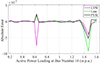 |
Figure 10 Absolute error in LVSI, Lmn, and FVSI indices of bus 14 for NR and ANN methods with heavy active power loading at bus 14. |
Comparison of LVSI, Lmn, and FVSI indices for NR and ANN methods with different active power loading at bus 14.
The result is extremely accurate, as shown in Table 3, and significant, with a best validation error of 8.9706e–08 and a minimum of epoch 329 for the test. The MSE obtained is of the order of 10e–8 in training and testing (Fig. 11). Figure 12 displays the fittings of the linear regression curve between the target and output. Also, the ANN training plot for the IEEE 14-bus system is shown in Figure 13.
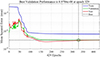 |
Figure 11 Curve between MSE and epochs for IEEE 14-bus system. |
 |
Figure 12 Regression plot between the output versus the target of training, validating, and testing for the IEEE 14-bus system. |
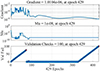 |
Figure 13 ANN training plot for IEEE 14-bus system. |
In a similar manner, ANN is developed for real and reactive power losses of the system and lines associated with the severe bus. For this, the active power loadings of bus 14 are considered as input data of the ANN. And corresponding real and reactive power losses of the lines (14-13) and (14-9), and the total real and reactive power losses of the test system are considered as target parameters. A total of 121 samples are taken using the NR method, out of which 91 and 30 samples are used for the training and testing of the ANN, respectively. The comparison of real and reactive power losses in the lines (14-13) and (14-9) obtained from NR and ANN methods under the different active power loading at bus 14 is shown in Table 4. Also, the total real and reactive power losses of the IEEE 14-bus test system evaluated from the NR and ANN methods are compared in Table 5. From Tables 4 and 5, it is observed that the results obtained from the offline NR approach and fast ANN approach are very close to each other.
Real and reactive power losses of the line (14-13) and (14-9) for NR and ANN methods with different active power loading at bus 14.
Real and reactive power losses of the IEEE 14-bus system for NR and ANN methods with different active power loading at bus 14.
The plot of the absolute error in the measurement of the real and reactive power losses of the system and in lines (14-13) and (14-9) by NR and ANN methods under different active power loading is shown in Figure 14. The value of this error is very small (order of 10e–4), which shows the predicted values of the real and reactive power losses by the ANN approach are very accurate.
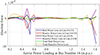 |
Figure 14 Absolute error in real and reactive power losses in the lines (14-13), (14-9), and IEEE 14-bus system for NR and ANN methods with heavy active power loading at bus 14. |
5.3.2 IEEE 118-bus system
The results of bus voltage indices of bus 14 at different active power loadings from the NR and ANN methods are shown in Table 6. To develop the ANN network for the bus voltage indices of the critical bus 44, the active power loading at bus 44 is considered as input data, and the LVSI, Lmn, and FVSI indices obtained from the NR method are considered as target data. A total of 104 samples are taken for the design of the ANN, and from that, 78 samples are taken for training the network, and 26 samples are considered for testing purposes. The variation of active power loading at bus 44 is considered from base load to maximum critical load. The absolute errors calculated between results obtained from the NR and ANN methods are in the order of 10e–4, which is very small. As evident from Table 6, the developed ANN is very efficient and accurate for forecasting the LVSI, Lmn, and FVSI indices of the most severe bus of the IEEE 118-bus system. Figure 15 shows the absolute error between the NR and the ANN method versus the active power loading curve.
 |
Figure 15 Absolute error in LVSI, Lmn, and FVSI indices of bus 44 for NR and ANN methods with heavy active power loading at bus 44. |
Comparison of LVSI, Lmn, and FVSI indices for NR and ANN methods with different active power loading at bus 44.
With the best validation error of 1.6461e–06 and a minimum at epoch 708 on the test set, the result is extremely accurate and significant, as shown in Table 6. In training and testing, the MSE was of the order of 10e–06 (Fig. 16). The fittings of the target vs output linear regression curve are shown in Figure 17. Additionally, Figure 18 displays the ANN training plot for the IEEE 118-bus system.
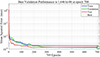 |
Figure 16 Curve between MSE and epochs for IEEE 118-bus system |
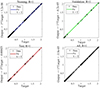 |
Figure 17 Regression plot between the output versus target of training, validating, and testing for the IEEE 118-bus system. |
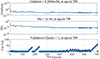 |
Figure 18 ANN training plot for IEEE 118-bus system. |
ANN is developed in a similar way for real and reactive power losses of the system and lines connected to the severe bus. The active power loadings of bus 44 are regarded in this as input data for the ANN. Furthermore, the corresponding real and reactive power losses of lines (44-43) and (44-45), as well as total real and reactive power losses for the test system, are taken into consideration as the target parameters. A total of 104 samples are collected using the NR method, of which 78 samples are used to test, and 26 samples are used to train the ANN. Table 7 illustrates the comparison of real and reactive power losses in lines (44-43) and (44-45) obtained from NR and ANN methods under base load to critical active power loading at bus 44. Additionally, Table 8 compares the total real and reactive power losses of the IEEE 118-bus test system as determined by NR and ANN methods. Tables 7 and 8 show that the results from the fast ANN approach and the offline NR approach are very similar to one another.
Real and reactive power losses of the line (44-43) and (44-45) for NR and ANN methods with different active power loading at bus 44.
Real and reactive power losses of the IEEE 14−bus system for NR and ANN methods with different active power loading at bus 14.
Figure 19 depicts the relationship between the absolute error in the measurements of the system’s real and reactive power losses, as well as in lines (44-43) and (44-45), using the NR and ANN methods under various active power loading conditions. The fact that this error is so small (of the order of 10e–4) demonstrates how accurately the ANN approach predicts the real and reactive power losses.
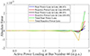 |
Figure 19 Absolute error in real and reactive power losses in the lines (44-43), (44-45), and IEEE 118-bus system for NR and ANN methods with heavy active power loading at bus 44. |
6 Conclusion
In this paper, the IEEE 14-bus and IEEE-118-bus systems are thoroughly examined to determine the effect of the active power load on the values of the indices as a function of the maximum load capability. A comparison between the traditional NR load flow and the ANN technique is presented to predict the bus voltage stability of the system under heavy active power loading. The feed-forward back-propagation ANN, which is based on the LM technique, is used to predict indicator values at load buses more quickly for the IEEE 14-bus and IEEE 118-bus systems. The accuracy of the Newton-Raphson and ANN methods together is found to be 99.99% or so. The result is extremely accurate, as shown in Tables 3–8, and significant, with the best validation error of 8.9706e–08 and 1.6461e–06, and a minimum of epoch 329 and 708 for the test of the IEEE 14-bus and IEEE 118-bus systems. The MSE obtained is of the order of 10e–08 and 10e–06 in training and testing for the IEEE 14-bus and IEEE 118-bus systems. Additionally, by identifying the voltage collapse point and the system’s weakest node, the optimal location for STATCOM using the LVSI, Lmn, and FVSI indicators based on critical loading conditions is demonstrated in this article. This helps to fortify the system and provides a strategic location for other compensation devices. The maximum loadability of the system can be evaluated by tracing the nose curve; in the future, the voltage stability of the system can be predicted by tracing the nose curve in online mode using Bessel’s function approach.
References
- Jayasankar V., Kamaraj N., Vanaja N. (2010) Estimation of voltage stability index for power system employing artificial neural network technique and TCSC placement, Neurocomputing 73, 16–18, 3005–3011. [Google Scholar]
- Princy U., Jaseena S., Sreedharan S., Sreejith S. (2017) Voltage stability analysis of power system network integrated with renewable source and SVC, in: 2017 Innovations in Power and Advanced Computing Technologies (i-PACT), IEEE, pp. 1–6. [Google Scholar]
- Kamalasadan S., Srivastava A.K., Thukaram D. (2006) Novel algorithm for online voltage stability assessment based on feed forward neural network, in 2006 IEEE Power Engineering Society General Meeting, p. 7. [Google Scholar]
- Puppala V., Chandrarao P. (2015) Analysis of continuous power flow method, model analysis, linear regression and ANN for voltage stability assessment for different loading conditions, Procedia Comput. Sci. 47, 168–178. [Google Scholar]
- Modarresi J., Gholipour E., Khodabakhshian A. (2016) A comprehensive review of the voltage stability indices, Renew. Sustain. Energy Rev. 63, 1–12. [CrossRef] [Google Scholar]
- Borazjani O., Roosta M., Isapour K., Rajabi A.R. (2015) Using artificial neural network algorithm for voltage stability improvement, Int. J. Electric. Comput Eng. 9, 3, 365–370. [Google Scholar]
- Jadhao C.W., Vadirajacharya K. (2015) Performance improvement of power system through static VAR compensator using sensitivity indices analysis method, in 2015 International Conference on Energy systems and applications, IEEE, pp. 200–202. [Google Scholar]
- Sharma A. (2016) Voltage stability assessment using GVSM and preventive control using SVC, Int. J. Comput. Appl. 142, 11. [Google Scholar]
- Chakrabarti S. (2008) Voltage stability monitoring by artificial neural networkusing a regression-based feature selection method, Expert Syst. Appl. 35, 4, 1802–1808. [Google Scholar]
- Ashraf S.M., Gupta A., Choudhary D.K., Chakrabarti S. (2017) Voltage stability monitoring of power systems using reduced network and artificial neural network. Int. J. Electr. Power Energy Syst. 87, 43–51. [Google Scholar]
- Sharma P., Ahuja R.K., Vashisth S., Hudda V. (2014) Computation of sensitive node for IEEE-14 bus system subjected to load variation, in Int. J. Innovative Res. Electric. Electron. Instrum. Control Eng. 2, 6, 1603–1607. [Google Scholar]
- Devaraj D., Roselyn J.P. (2011) Online voltage stability assessment using radial basis function network model with reduced input features, Int. J. Electr. Power Energy Syst. 33(9), 1550–1555. [Google Scholar]
- Subramani C., Jimoh A., Kiran S.H., Dash S.S. (2016) Artificial neural network-based voltage stability analysis in power system, in 2016 International Conference on Circuit, Power and Computing Technologies (ICCPCT), IEEE, pp. 1–4. [Google Scholar]
- Goh H., Chua Q., Lee S., Kok B., Goh K., Teo K. (2015) Evaluation for voltage stability indices in power system using artificial neural network, Procedia Eng. 118, 1127–1136. [Google Scholar]
- Singh P., Parida S.K., Chauhan B., Choudhary N. (2020) Online Voltage stability assessment using artificial neural network considering voltage stability indices, in 2020 21st National Power Systems Conference (NPSC), Gandhinagar, India, pp. 1–5. https://doi.org/10.1109/NPSC49263.2020.9331954. [Google Scholar]
- Aydin F., Gümüş B. (2020) Study of different ANN algorithms for voltage stability analysis, in 2020 Innovations in Intelligent Systems and Applications Conference (ASYU), Istanbul, Turkey, pp. 1–5. https://doi.org/10.1109/ASYU50717.2020.9259817. [Google Scholar]
- Kumar S., Tyagi B., Kumar V., Chohan S. (2022) PMU-based voltage stability measurement under contingency using ANN, IEEE Trans. Instrum. Measure. 71, 1–11. Art. No. 9000111. https://doi.org/10.1109/TIM.2021.3129210. [CrossRef] [Google Scholar]
- Zhang C., Mijatovic N., Cai X., Dragičević T. (2022) Artificial neural network-based pole-tracking method for online stabilization control of grid-tied VSC, IEEE Trans. Indus. Electron. 69, 12, 13902–13909. https://doi.org/10.1109/TIE.2021.3134079. [Google Scholar]
- Chettibi N., Massi Pavan A., Mellit A., Forsyth A.J., Todd R. (2021) Real-time prediction of grid voltage and frequency using artificial neural networks: An experimental validation, Sustain. Energy Grid. Netw. 27, 100502. [Google Scholar]
- Veerasamy V., Abdul Wahab N.I., Ramachandran R., Othman M.L., Hizam H., Devendran V.S., Irudayaraj A.X.R., Vinayagam A. (2021) Recurrent network-based power flow solution for voltage stability assessment and improvement with distributed energy sources. Appl. Energy 302, 117524. [Google Scholar]
- Amroune M. (2021) Machine learning techniques applied to on-line voltage stability assessment: a review, Arch. Computat. Methods Eng., 28, 273–287. https://doi.org/10.1007/s11831-019-09368-2. [Google Scholar]
- Saha G., Chakraborty K., Das P. (2022) Enrichment of voltage stability in power system through novel generalized approximate reasoning based intelligent control with African buffalo optimization approach, Soft Comput. 27, 7473–7496. https://doi.org/10.1007/s00500-022-07688-3. [Google Scholar]
- Yadav A.N., Pal K. (2022) Demand side maximum loading limit ranking based on composite index using ANN, Int. J. Syst. Assur. Eng. Manag. 13, 1419–1429. [Google Scholar]
- Hiremath R., Moger T. (2022) Grid-connected DFIG driven wind system for low voltage ride through enhancement using neural predictive controller, J. Inst. Eng. India Ser. B 103, 1577–1588. https://doi.org/10.1007/s40031-022-00761-3. [Google Scholar]
- Alimi O.A., Ouahada K., Abu-Mahfouz A.M. (2020) A review of machine learning approaches to power system security and stability, IEEE Access 8, 113512–113531. https://doi.org/10.1109/ACCESS.2020.3003568. [Google Scholar]
- Kessel P., Glavitsch H. (1986) Estimating the voltage stability of a power system, IEEE Trans. Power Delivery 3, 346–354. [Google Scholar]
- Gupta S.K., Mallik S.K., Tripathi J.M., Sahu P. 2021 Comparison of voltage stability index with optimal placement of SSSC considering maximum loadability, in 2021 International Symposium of Asian Control Association on Intelligent Robotics and Industrial Automation (IRIA), Goa, India, pp. 1–6. https://doi.org/10.1109/IRIA53009.2021.9588759. [Google Scholar]
- Moghavvemi M., Omar F.M. (1998) Technique for contingency monitoring and voltage collapse prediction. IEE Proc Gen. Trans. Distrib. 145, 6, 634–640. https://doi.org/10.1049/ipgtd:19982355. [Google Scholar]
- Musirin I., Rahman T.K.A. (2002) Online voltage stability based contingency ranking using fast voltage stability index (FVSI), in Proceedings IEEE/PES Transmission Distribution and Exhibition Conference, Vol. 2, pp. 1118–1123. [Google Scholar]
- Mohamed A., Jasmon G.B., Yusoff S. (1989) A static voltage collapse indicator using line stability factors, J. Indus. Technol. 7, 73–85. [Google Scholar]
- Ratra S., Tiwari R., Niazi K.R. (2018) Voltage stability assessment in power systems using line voltage stability index, Comp. Electric. Eng. 70, 199–211. [Google Scholar]
- Adetokun B.B., Muriithi C.M., Ojo J.O. (2020) Voltage stability assessment and enhancement of power grid with increasing wind energy penetration, Int. J. Electric. Power Energy Syst. 120, 105988. [Google Scholar]
All Tables
Line indices values of load buses of IEEE 14-bus under the critical active power loading.
Line indices values of load buses of IEEE 118-bus under the critical active power loading.
Comparison of LVSI, Lmn, and FVSI indices for NR and ANN methods with different active power loading at bus 14.
Real and reactive power losses of the line (14-13) and (14-9) for NR and ANN methods with different active power loading at bus 14.
Real and reactive power losses of the IEEE 14-bus system for NR and ANN methods with different active power loading at bus 14.
Comparison of LVSI, Lmn, and FVSI indices for NR and ANN methods with different active power loading at bus 44.
Real and reactive power losses of the line (44-43) and (44-45) for NR and ANN methods with different active power loading at bus 44.
Real and reactive power losses of the IEEE 14−bus system for NR and ANN methods with different active power loading at bus 14.
All Figures
|
Figure 1 A schematic illustration of STATCOM using two bus systems. |
| In the text | |
|
Figure 2 ANN network. |
| In the text | |
|
Figure 3 Flow chart of the proposed approach. |
| In the text | |
|
Figure 4 (a) Line indices LVSI, Lmn, FVSI, and bus voltage magnitude of bus 14 vs active power loading at bus 14. (b) Bus voltage magnitude of bus 14 with and without STATCOM under heavy active power loading at bus 14. |
| In the text | |
|
Figure 5 (a) Line indices LVSI, Lmn, FVSI, and bus voltage magnitude of bus 44 vs active power loading at bus 44. (b) Bus voltage magnitude of bus 44 with and without STATCOM under heavy active power loading at bus 44. |
| In the text | |
|
Figure 6 Real and reactive power losses of the lines (14-13) and (14-9). |
| In the text | |
|
Figure 7 Total real and reactive power losses of the IEEE 14-bus system. |
| In the text | |
|
Figure 8 Real and reactive power losses of the lines (44-43) and (44-45). |
| In the text | |
|
Figure 9 Total real and reactive power losses of the IEEE 118-bus system. |
| In the text | |
|
Figure 10 Absolute error in LVSI, Lmn, and FVSI indices of bus 14 for NR and ANN methods with heavy active power loading at bus 14. |
| In the text | |
|
Figure 11 Curve between MSE and epochs for IEEE 14-bus system. |
| In the text | |
|
Figure 12 Regression plot between the output versus the target of training, validating, and testing for the IEEE 14-bus system. |
| In the text | |
|
Figure 13 ANN training plot for IEEE 14-bus system. |
| In the text | |
|
Figure 14 Absolute error in real and reactive power losses in the lines (14-13), (14-9), and IEEE 14-bus system for NR and ANN methods with heavy active power loading at bus 14. |
| In the text | |
|
Figure 15 Absolute error in LVSI, Lmn, and FVSI indices of bus 44 for NR and ANN methods with heavy active power loading at bus 44. |
| In the text | |
|
Figure 16 Curve between MSE and epochs for IEEE 118-bus system |
| In the text | |
|
Figure 17 Regression plot between the output versus target of training, validating, and testing for the IEEE 118-bus system. |
| In the text | |
|
Figure 18 ANN training plot for IEEE 118-bus system. |
| In the text | |
|
Figure 19 Absolute error in real and reactive power losses in the lines (44-43), (44-45), and IEEE 118-bus system for NR and ANN methods with heavy active power loading at bus 44. |
| In the text | |
Current usage metrics show cumulative count of Article Views (full-text article views including HTML views, PDF and ePub downloads, according to the available data) and Abstracts Views on Vision4Press platform.
Data correspond to usage on the plateform after 2015. The current usage metrics is available 48-96 hours after online publication and is updated daily on week days.
Initial download of the metrics may take a while.