")
")
| Issue |
Sci. Tech. Energ. Transition
Volume 81, 2026
|
|
|---|---|---|
| Article Number | 13 | |
| Number of page(s) | 12 | |
| DOI | https://doi.org/10.2516/stet/2026013 | |
| Published online | 21 April 2026 | |
Regular Article
A hybrid PSO-LSTM-based electricity prediction and optimization technique for home appliances
1
Chitkara University Institute of Engineering and Technology, Chitkara University, Punjab, India
2
Thapar Institute of Engineering and Technology, Patiala, India
3
National Institute of Technology, Kurukshetra 136119, Haryana, India
* Corresponding author: This email address is being protected from spambots. You need JavaScript enabled to view it.
Received:
11
May
2024
Accepted:
23
February
2026
Abstract
With population growth and technological advancements, electricity demand in residential buildings has increased sharply. Accurate energy consumption forecasting enables building owners and operators to understand and predict the energy usage patterns of their buildings. However, the prevailing forecasting techniques have certain limitations that must be addressed for improved energy optimization. To address these concerns, this paper proposes a novel three-stage energy optimization framework for individual home appliances. In the first stage, season-wise cluster analysis is performed using a hierarchical clustering algorithm. In the second stage, an adaptive Long Short-Term Memory (LSTM) model is developed to estimate the electricity consumption of home appliances. Next stage integrates Particle Swarm Optimization (PSO) for hyperparameter tuning of the LSTM model to improve prediction accuracy. Then, the hybrid PSO-LSTM technique has been rigorously evaluated using a benchmark dataset on energy consumption of individual home appliances. Comparative analysis with previous state-of-the-art prediction models reveals the superiority of the proposed work. Integration of clustering, deep learning, and optimization offers a practical solution for smart energy management. The extracted insights show that the proposed approach leads to sustainable, efficient, and user-aware energy practices in households.
Key words: Cluster analysis / Deep learning / Energy prediction / Optimization / Home appliances
© The Author(s), published by EDP Sciences, 2026
 This is an Open Access article distributed under the terms of the Creative Commons Attribution License (https://creativecommons.org/licenses/by/4.0), which permits unrestricted use, distribution, and reproduction in any medium, provided the original work is properly cited.
1 Introduction
Electricity demand is rapidly growing in different sectors, namely residential and commercial buildings, industry, transport, and agriculture. According to reports from the International Energy Agency (IEA) [1], energy consumption in residential buildings has largely increased. The primary contributors to rising electricity consumption in the residential sector are the rising population and the availability of domestic appliances at nominal prices. Energy consumption and generation must be aligned, as they cannot be stored or transported. Technological advancements have adopted the IoT paradigm in buildings for energy management. IoT devices, including smart meters and sensors, are generating large time-series data that are useful for demand-side energy estimates. The increased energy consumption motivated the researchers to develop strategies for energy prediction and optimization. Precise estimates are beneficial for electricity suppliers, utility companies, and consumers [2, 3]. Therefore, overestimation can lead to monetary losses, and underestimates may result in a shortage of power [4]. There are various factors, namely, the number of occupants, outdoor temperature, humidity, building design parameters, and usage behavior, influence the electricity consumption prediction performance [5].
Machine learning, as well as deep learning-based prediction models, have been developed to estimate the energy demand of residential buildings [6, 7]. Deep learning models performed excellently and achieved high accuracy, as these models can better handle non-linear data [8, 9], in comparison to classical models. Indeed, the performance of deep learning models is affected by certain hyperparameter values [10]. To deal with hyperparameter selection, various optimization approaches are available that make the hyperparameter selection automatic [11]. It will reduce the error rate while improving the prediction accuracy of deep learning models. The hyperparameter selection techniques, such as grid search, swarm intelligence, and evolutionary algorithm, are utilized by several authors for optimizing the performance. As a result, the optimization approaches improved accuracy, but there is still a scope for improvement, and the existing energy prediction techniques are underperforming heterogeneous home appliances due to varying consumption patterns and operational features. In this paper, a hybrid electricity forecasting approach has been implemented by integrating an LSTM model and a PSO approach. The PSO is employed to optimize the model’s hyperparameters (neuron units, learning rate, and batch size) to improve the model’s accuracy and convergence. Further, this combined energy prediction and optimization approach has been applied to make predictions using the energy consumption dataset of home appliances. The results analysis shows that the proposed PSO-LSTM-based prediction approach reduced the prediction error in comparison to existing prediction models. The proposed approach can potentially provide consumers with awareness and understanding of their usage patterns of home appliances. The research contributions of this paper are mentioned as follows.
1.1 Motivation and our novel contributions
-
The fluctuating climatic conditions highly impact the energy utilization of a particular set of home appliances [12, 13]. The proposed work performs cluster analysis based on the whole-year weather conditions using the Agglomerative Hierarchical Clustering (AHC) algorithm.
-
A LSTM model has been trained and tested on heterogeneous home appliances by incorporating the usage patterns to improve the prediction performance [9].
-
To handle dissimilarities of electricity-driven appliances, an LSTM model is built separately based on optimized hyperparameters [5]. The hyperparameters, namely, time_step, neuron_units, and batch_size, are optimized using a Particle Swarm Optimization (PSO) approach.
-
The performance of the hybrid PSO-LSTM approach has been verified on a benchmark dataset of individual home appliances and compared with state-of-the-art works.
This paper follows the structure: Section 2 discusses the related literature in the field of prediction and optimization, followed by the material and methods section. Further, Section 3 elaborates on the methodology of the proposed work, and experimental results are discussed in Section 4. Finally, Section 5 concludes the proposed hybrid PSO-LSTM approach.
2 Related work
The literature survey elaborates on the existing research papers on machine learning and deep learning-based prediction approaches. The popular prediction models developed by several authors are Random Forest (RF), Support Vector Regression (SVR), ensemble models, and neural network models [13, 14]. The household appliances have been categorized by many authors using clustering algorithms [15, 16] to fetch day-wise energy consumption patterns. Satre-Meloy et al. [17] have developed a clustering-based demand forecasting approach to extract peak demand hours using k-means and hierarchical clustering. Abera and Khedkar [18] proposed an ensemble XGBoost model to classify and predict peak energy demand of residential buildings. Petsis et al. [19] developed an Ensemble prediction model using RF and SVM for estimating the indoor temperature of smart homes. Wang et al. [20] proposed an edge computing-based energy management framework for residential buildings. The indoor temperature is being controlled by an automatic learning algorithm. Piscitelli et al. [21] applied ANN and RT models to estimate the energy consumption patterns on University campuses. The authors have detected abnormal patterns of energy consumption; the performance was verified using a benchmark dataset.
Ngo et al. [22] developed prediction models using an ensemble model for non-residential buildings future energy demand. Authors applied ANN, SVR, and M5Rules models and found that the ensemble approach outperformed and accurately predicted energy demand. Khan et al. [3] developed a short-term energy prediction and optimization approach. Authors have used LSTM and Gated Recurrent Unit (GRU) for predictive analytics and also applied K-means clustering to arrange apartment-wise consumption patterns. The proposed work successfully achieved a small error rate; in the future, this approach can be implemented and extended onto large datasets. Similarly, Kim and Cho [23] proposed CNN-LSTM and autoencoder-based energy prediction models for residential buildings. Theogene Bimenyimana [24] proposed a load forecasting architecture using RF and LSTM models for the residential sector using weather information. The experimentation was performed using the AMPds dataset.
Ilbeigi et al. [25] developed an energy prediction and optimization technique based on NN and GA for office buildings. The objective function is taken as energy consumption, which was optimized using GA. The proposed approach has reduced the average energy consumption by 35% on the simulated dataset of EnergyPlus and the Grasshopper tool. Another optimization approach based on the adaptive Grey Wolf Optimization (GWO) algorithm was proposed by Li et al. [26] to predict indoor temperature level of residential buildings and energy consumption. Later, Wang et al. [27] developed a load forecasting approach using GRU for smart appliances in households. The prediction accuracy of the proposed framework has been assessed using benchmark datasets, namely, AMPds, UKDALE, and DRED. Besides, Sauer et al. [28] combined Jaya optimizer with eXtreme Gradient Boosting (XGBoost) to estimate the energy demand of residential buildings.
The summary of existing prediction models is extracted and specified in Table 1. It has been analyzed that energy prediction models deployed in residential and other buildings are based on machine learning and deep learning techniques. Few authors have applied weather clustering by considering smart home appliances. The performance has been evaluated using benchmark, simulated, or real-time energy consumption datasets. As per the literature review, some research works are integrating weather clusters to extract seasonal patterns in energy consumption for smart homes.
Summary of energy consumption prediction and optimization models developed in the literature in comparison to the proposed work.
2.1 Research gaps
The following research gaps have been found during the literature review:
-
Several authors have predicted the whole building’s energy consumption instead of considering the individual home appliances [37, 39]. It may not provide granular details related to household energy consumption patterns. The energy usage of specific home appliances is influenced by weather conditions [9, 38], and few authors have considered changing weather conditions when predicting the energy demand of home appliances.
-
Few authors have associated weather conditions with whole building energy consumption [40]. However, the energy consumption of home appliances is not clustered according to the different seasons of the year.
-
Some authors have utilized neural network-based models for energy prediction of residential buildings [41], but clustering algorithms need to be integrated with prediction models.
3 Techniques used
In this paper, a hybrid prediction approach is proposed, considering the weather conditions throughout the year using clustering and regression analysis. An optimization technique known as particle swarm optimization is adopted for hyperparameter selection of a deep learning model. The methods and techniques used in this paper are discussed subsequently.
3.1 Agglomerative Hierarchical Clustering (AHC)
An unsupervised learning technique, clustering is useful to group or segregate the dataset into homogeneous subsets based on a similarity index. It provides a deeper understanding of unknown patterns in the dataset. There exist various clustering algorithms, such as k-means, DBSCAN, hierarchical, etc., that extract similar clusters based on similarity measures or apply some grouping criteria. But k-means depends on the prior information about the number of clusters, and DBSCAN depends on sensitive density parameters; in contrast, hierarchical clustering is a non-parametric technique that searches naturally occurring seasonal clusters in time-series data. The dendrogram offers cluster selection, showing the number of clusters at various levels, capturing subtle changes in seasonal appliance usage.
This research work applied an agglomerative hierarchical clustering approach. In this method, each data point is considered as a single cluster, and the model keeps identifying the remaining data points and adds them to the appropriate cluster based upon the distance between the data points [17]. The distance measure and linkage method used in this paper are discussed below.
-
For time-series data, the famous distance measure known as dynamic time warping (DTW) is used. It calculates the distance more accurately compared to the Euclidean distance method, as data is arranged in a time-sequential order [42]. DTW computes the distance between data points and selects the data points with the shortest distance.
-
The similarity between different clusters is found using Ward’s linkage criterion method. Based upon this, the similar data points are added to the same cluster [13]. The Ward’s method is useful to avoid large cluster formation, and requires no prior knowledge of the number of clusters required.
The closest clusters are combined into one cluster. This process is repeated until all similar clusters are converged. Subsequently, similar clusters are merged in every iteration until a big cluster consists of all data points. Eventually, the clustering algorithm identifies the significant climatic patterns in the electricity consumption of home appliances.
3.2 Long short-term memory unit model
LSTM is suitable for solving time-series prediction problems because it can remember the historical data for a long time. LSTM is a type of Recurrent Neural Network (RNN) which is able to preserve only short-term information across data points, addressing the problem of vanishing gradient points [43]. The information can be retained over a longer period of time through a set of layers called cell states that save the historical data [44], and the issue of vanishing gradient point is resolved in the LSTM neural network. Additionally, it consists of three other components, namely: the forget gate, input gate, and output gate, shown in Figure 1 [45].
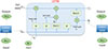 |
Figure 1 Architecture of the LSTM network. |
The new electricity data Xt enters into the input gate at time-stamp t, and the forget gate ft keeps the historical data, and both are combined for updating the previous cell state ct − 1 to the subsequent cell state ct. Further, the state information is utilized to generate the output; this information is filtered by output gates, hidden layers, and the desired output Yt is produced at the end.
3.3 Particle swarm optimization approach
Particle swarm optimization is a swarm intelligence-based meta-heuristic technique that is commonly used to solve non-linear objective functions [46]. It follows the bird’s behavior adopted for food search. According to the position of the neighbor, the birds change their position to fit in the best position. The birds are called particles, characterized by speed, location, and fitness value computed with a fitness function. The particles drift their trajectory to find the optimum spot. The updated location (position) and speed of particles are calculated using equations (1) and (2) defined below: (1)
(1)
 (2)where
  is the rate of change of particles’ position, W is the inertia weight, c1, c2 are the position constants, and r1, r2 are the random numbers selected uniformly within [0, 1]. Where i = 1, 2, 3 … N (N is the ith particle), j = 1, 2, 3… M (M is the search space dimension), local best and global best particles are depicted as pbest and gbest. The particle population is optimized for candidate solutions, the particles are directed to the open search space using new positions, and the velocity of particles. Varying the dimensions and PSO particles can enhance the convergence rate and computational complexity. The present work applies PSO for the LSTM model’s hyperparameter selection.
The techniques mentioned in this section are employed to design an energy prediction framework for smart appliances in households. The subsequent section presents the proposed methodology adopted for this research work.
4 Proposed methodology: Hybrid PSO-LSTM-based technique
The proposed hybrid technique for prediction and optimization of energy consumption for implementing the energy-aware prediction model is depicted in Figure 2. It comprises three primary modules: data preprocessing, data clustering, energy prediction, and optimization approach. The subsequent section elaborates all three modules in systematic order.
 |
Figure 2 Proposed hybrid PSO-LSTM-based prediction and optimization approach for home appliances. |
4.1 Dataset description and preprocessing
In the proposed work, the smart meters’ electricity consumption dataset, known as the Almanac of Minutely Power data set (AMPds), has been utilized [47]. The AMPds dataset is a collection of electricity consumption recorded from a single house in Greater Vancouver for a period of two years. There are overall 1048575 rows measured at 1-minute time intervals using UNIX-timestamp for each sub-meter electricity consumption.
This paper uses five home appliances or loads, namely, Furnace/HVAC (FRE), Hot water unit (HTE), Refrigerator (FGE), Heat pump (HPE), and Clothes dryer (CDE). The selected appliances fall into the category of high energy-consuming, but the appliances such as plugs and lights, which are low energy-consuming appliances, are not taken for model training. In the proposed work, the actual power consumption of five home appliances is depicted in Table 2. The Watt is a unit of actual power consumption, and the data of electricity measurements is stored as a CSV file format. All these appliances exhibit different usage patterns.
Description of home appliances for AMPds.
Search space parameters of PSO algorithm.
Appliance-wise optimized hyperparameters given by the PSO algorithm for LSTM model training.
Predictive performance of proposed PSO-LSTM prediction model for individual home appliances.
Comparative analysis with existing prediction approaches.
Data preprocessing is applied to prepare the input data for model training. The electricity data is stored in UNIX-timestamp order, which is converted into a date-time format. The input dataset contains missing values that need to be filled. Therefore, linear interpolation is applied, and the missing values are filled with the average of the previous and next value in the sequence. Hence, the missing value is computed and filled with the same sequence of prior values. To detect outliers in the input dataset, we have performed data visualization, and some outlier values are found to have a skewed distribution. The interquartile range method (IQR) is applied to treat outliers. Then the energy measurements recorded on a minute interval are resampled into the day-wise energy data. Later, we applied data transformation using the Min-Max scalar given by the equation (3) [48]. The min-max scalar transforms the input datapoints into the range of (0, 1). (3)
(3)
4.2 Data clustering
The season-wise clustering has been performed to create energy clusters. The individual home appliances’ energy consumption trend during various climatic conditions throughout the year has been investigated. We have considered four seasons, i.e., summer, winter, autumn, and spring, for trend analysis. We have applied agglomerative hierarchical clustering to fetch month-wise energy clusters and to analyze year-round usage patterns of various home appliances. The clustering process begins with the initial n energy measurements and creates individual clusters iteratively by combining similar clusters. The dynamic time-warping (DTW) method is used to compute the similarity of two clusters based on the shortest distance between two data points. depicted by distance D(p, q) is the minimum value between the two data points p(p1, p2, p3, p4…pi) and q(q1, q2, q3, q4 … qj) is given by equation (4):![Mathematical equation: $$ D\left(p,q\right)=\left|{p}_i-{q}_j\right|+\mathrm{min}D\left[i-1,j-1\right],D\left[i-1,j\right],D\left[i,j-1\right]. $$](/articles/stet/full_html/2026/01/stet20240132/stet20240132-eq5.gif) (4)
(4)
A new cluster is produced by merging similar clusters, and data in the distance matrix is updated after each iteration. The data cluster are representation of season-wise energy consumption throughout the year for a particular appliance dataset. The season-wise clusters of appliance energy consumption are shown in Figure 3, showing consumption patterns of appliance energy demand in various seasons. The energy consumption of the AMPDS dataset reveals that the climatic conditions of Canada comprise four seasonal clusters. Where Cluster 1 is clearly seen as distributed in the winter season across late December, January, February, March, and April. While Cluster 2 is spread in the months of the spring season, i.e., late April, May, and June, and Cluster 3 is distributed across the summer season months, July, August, and September. Eventually, cluster 4 consists of autumn months, namely late September, October, and November. The changing weather conditions throughout the year affect the performance of energy consumption prediction. In the next section, a hybrid prediction and optimization model has been developed to predict appliance-wise energy consumption.
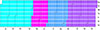 |
Figure 3 Season-wise energy clusters for year-round historical data. |
4.3 Hybrid PSO-LSTM-based prediction and optimization technique
The main aim of cluster analysis is to identify meaningful patterns in energy consumption and to provide day-wise (timestamp) and season-wise energy clusters for predicting electricity demand in the future.
The proposed hybrid approach utilized a univariate LSTM model to predict the energy consumption of individual home appliances. However, LSTM model performance is influenced by a certain set of hyperparameters; this paper adopted a swarm intelligence-based PSO algorithm for optimal hyperparameter selection. Here, PSO is implemented for choosing hyperparameters, namely, time_step, neuron_units, and batch_size. These parameters are considered as decision variables in the optimization process by taking the mean absolute error (MAE) as the objective function. The proposed hybrid optimization approach is depicted in Figure 4 (Algorithm 1).
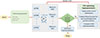 |
Figure 4 Proposed workflow of hybrid PSO-LSTM approach for hyperparameter optimization. |
Input: Households electricity consumption dataset (E)
Output: Energy predictions
1: Initialization: Hyperparameters time_step, neuron_units batch_size and swarm
2: Initialization of fitness_function (MAE)
3: Declare personal and global best particle p_best, p_gbest
4: train and test sets split
5: build LSTM model
6: update particle velocity using p_best and p_gbest
7: use velocity to compute particle position
8: Evaluate fitness_score ←MAE
9: If max_iteration <= 50 then
10: goto step 5
11: end if
12: model.predict(test_x)
13: Calculate loss = MAE
Initially, the hyperparameters time_step, neuron_units, and batch_size are declared and initialized; subsequently, the swarm and fitness function (MAE) are initialized. Next, the local and global particles are initiated and updated. The list of hyperparameters selected for optimization is specified in Table 3. The swarm size selection is a crucial step because a small swarm size may lead to a solution that gets stuck at a local space, failing to reach the global solution; in contrast, a large swarm size achieves an optimal solution, consuming high resources. The optimal global solution is found after evaluation of the fitness function for each LSTM model trained for an individual home appliance. The hyperparameters search starts with a random set of particles. We have used the trial-and-error method for selecting the swarm size and the inertia weight parameters during model training. The best swarm size and inertia weight vary in the case of heterogeneous data. The optimal global solution yielded within the range of ns ∈ [10, 20] for the optimal swarm size ns. The inertia weight (ω) is set at ω ∈ [0.9]. The acceleration constants, C1 and C2, are assigned values 0.5 and 0.3, respectively, whereas the random number r1 and r2 are taken as 0.8 and 0.3, respectively.
The predictive analysis LSTM model has been done using the performance metric MAE. LSTM model takes a three-dimensional matrix in which the input data’s size is the first dimension, timestamps are the second dimension, and the number of output observations is the last dimension. In this research, input electricity dataset is converted into a supervised dataset. We have applied the lag window method to transform time series signals into a supervised learning dataset, generating lag observations of column energy consumption. The updated three-dimensional dataset consists of matrix with multiple inputs  produced by function
  where
where  is an input energy dataset,
  is the past day timestamp and
  is the next day timestamp showing predicted energy demand.
4.4 Performance metrics
To evaluate the performance of the hybrid energy prediction and optimization model, we have computed state-of-the-art metrics such as MAE, mean squared error(MSE), and root mean squared error (RMSE). These performance metrics are defined below in equation (5): (5)where energy data points are denoted as
  , the target value is depicted as
  and the predicted outcome is denoted by
  for each appliance dataset.
5 Experimental results
The proposed hybrid energy prediction model is evaluated on a benchmark dataset, i.e., AMPds [47], which is a collection of individual home appliances. We have used Python 3, using Keras with TensorFlow to develop an electricity prediction approach. PySwarm, a Python-based research tool, is applied for PSO hyperparameter optimization. The PSO algorithm takes a particle population, including velocity and position, repeat the optimization process until optimal parameters are achieved. The optimal hyperparameters are used for LSTM model training for each home appliance dataset. The appliance-wise dataset has been divided into a training and a testing. The LSTM model contains one hidden layer and ‘relu’ is taken as the activation function, followed by one dense layer for producing output. Adam optimizer is used to build the model, and Mean Absolute Error calculates the loss function. Then the proposed model is trained and tested for 50 epochs.
5.1 Predictive performance of novel PSO-LSTM-based technique
The hybrid PSO-LSTM model has been deployed to predict the energy consumption of individual home appliances. We have entered the day-wise energy consumption record, which is assigned to a vector xt; t depicts the timestamp of the day. Further lagged window converted it into a vector comprising previous days’ timestamps. For the LSTM model, specific hyperparameters such as input lag value, number of neurons, and batch size are searched using a PSO-based optimization approach. The home appliances are characterized as heterogeneous and non-linear in consumption behavior. Therefore, every appliance shows different consumption trends during specific hours, on certain weekdays, and months. The LSTM model performance is generalized by the PSO approach, and adaptive LSTM architectures are implemented for smart home appliances. Table 4 depicts appliance-wise optimized hyperparameters given by the PSO algorithm.
The hybrid prediction model is trained to estimate the next day’s energy demand. The prediction accuracy is measured using performance metrics, namely MAE, MSE, and RMSE. Figure 5 depicts different home appliances’ energy predictions and actual energy consumption. The x-axis and y-axis represent the number of measurements and the amount of electricity consumed by particular home appliances. The blue lines in the graph depict actual measurements, and the orange lines represent predicted values. The proposed work successfully attained generalized results for heterogeneous home appliances. At certain points, input data contains non-stationary and fluctuating patterns, which is the reason behind the difference between actual and predicted energy consumption.
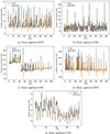 |
Figure 5 Energy predictions of individual home appliances. |
FGE is a finite-state-type appliance, and the consumption patterns are high peak values, as shown in Figure 5b therefore, accurate energy consumption predictions are obtained. The load of home appliances CDE is a finite-state, depicting peak values on some days, and the model received close energy predictions Figure 5c. However, the consumption patterns of the HPE and HTE appliances exhibit fluctuation, which results in gaps between the actual and predicted values. Eventually, the proposed hybrid model obtained close electricity predictions as shown in Figure 5d, Figure 5a. The proposed model has achieved close predictions as compared to actual measurements for a constant load type home appliance FRE (Furnace/HVAC) as shown in Figure 5c.
We have trained and tested a standalone LSTM model without hyperparameter optimization and a hybrid LSTM model using PSO-optimized hyperparameters. The performance of both LSTM and hybrid PSO-LSTM approaches has been verified and compared. In the case of the LSTM model, the minimum MAE value (0.125 kWh) is attained on the CDE dataset, and the maximum MAE value (0.183 kWh) is obtained on the HTE dataset. The prediction results for both the LSTM and the hybrid PSO-LSTM model are presented in Table 5. PSO-LSTM provides the minimum MAE (0.105 kWh) using the refrigerator (FGE) dataset. However, the maximum MAE (0.152 kWh) has been achieved on the instant hot water unit(HTE) dataset.
5.2 Statistical analysis
In this paper, we performed a statistical test to verify the performance of the model. The proposed work applies the Wilcoxon signed-rank test to all datasets of individual home appliances for LSTM and PSO-LSTM model prediction results [49]. This test compares the performance of two related machine learning models using MAE, MSE, and RMSE on individual appliance datasets. Then the performance differences for each case are arranged and ranked. For these metrics, the Wilcoxon test has been performed to evaluate whether this median difference lies between 0 and 0.05. It has been found that the p-value falls within the range of 0.05 for all metrics, which shows PSO-LSTM improved prediction performance compared to the LSTM model.
5.3 Comparative analysis with existing approaches
The AMPds dataset [50] is used to compare how well the hybrid PSO-LSTM technique can make predictions with other machine learning models and neural network-based models. The comparative analysis with existing research papers is given by Table 6. The authors [12] have implemented clustering on individual appliances for predicting the energy demand of appliances within each cluster. They have applied an ANN model for prediction and obtained RMSE (2.55 kWh). Gajowniczek and Ząbkowski [13] used the same energy consumption dataset (AMPds) to forecast future energy consumption by training a neural network model and provided an MAE of 0.23 kWh. In another paper, Hossen et al. [9] trained an LSTM model on the AMPds dataset [50] to predict energy consumption and attained MAE (0.24 kWh). The comparative result analysis reveals that the proposed PSO-LSTM model outperformed the existing prediction model.
5.4 Computational overhead and complexity analysis
During LSTM model training, hyperparameters are selected manually using the hit-and-trial method. In contrast, the PSO-based hyperparameter selection approach has been adopted for LSTM. Although the computational overhead of PSO-LSTM has increased due to the optimization process. The PSO has P number of particles and I number of iterations, which contributes to the increased training time with a factor of P × I, because for all configuration settings, model training is being performed. However, computational overhead can be ignored if it achieves improvement in prediction performance with minimum external intervention. In certain scenarios, such as limited computational resources, the PSO parameters can be calibrated by reducing the swarm size or number of iterations.
5.5 Implications and Limitations
The proposed hybrid PSO-LSTM technique is suitable for implementing energy management for household appliances in residential structures. Additionally, it might be advantageous for homes, as it increases user awareness by presenting daily energy use patterns. The season-wise cluster analysis reveals the usage trends of particular home appliances across seasons throughout the year.
Also, this component enables utility companies and energy management teams to develop adaptive demand-response policies based on seasonal consumption patterns that can improve grid reliability and encourage load shifting during peak hours. Besides, the hybrid prediction model can be integrated with IoT-based smart meters to design a home automation system, providing actionable recommendations on the consumer dashboard in real-time.
It is important to take into account human behavior when developing energy prediction models for residential appliances. Thus, it is necessary to have a dataset that specifically captures the occupancy and energy-usage patterns of different equipment in residential structures. The present work has been tested on residential buildings; its performance evaluation on commercial, educational, and industrial buildings is unexplored. To assess the applicability and reliability of the PSO-LSTM-based technique, it can be implemented on various categories of residential and commercial buildings that exhibit unique consumption patterns. The efficacy of the suggested method relies on both the amount and the caliber of the input dataset. Additionally, it is necessary to provide a user-friendly interface that offers real-time data on energy consumption.
6 Conclusion
This paper proposed a hybrid electricity prediction and optimization technique for home appliances using LSTM and PSO. Initially, each appliance with identical energy consumption behavior is categorized as a seasonal cluster using a hierarchical clustering algorithm. Secondly, the hybrid PSO-LSTM model is developed with PSO-optimized hyperparameters. Next step, deploys the proposed PSO-LSTM technique on individual home appliances to predict the next day’s electricity demand. The results of the experiment unequivocally demonstrate that the choice of hyperparameters for the LSTM model is crucial, as it has a direct impact on the accuracy of predictions. The comparative investigation demonstrates that the PSO-LSTM model has achieved an approximately 53% reduction in MAE in comparison to the LSTM model. In the future, the hybrid PSO-LSTM approach can be used on large-scale, real-time datasets of energy use to better anticipate electricity demand in homes. The framework can also be used in self-managing energy systems that not only provide real-time advice on appliance operation, but also recommend that users control the energy consumption. This kind of extension would make the proposed approach more useful in smart grid settings and help with sustainable energy management.
References
- IEA. 2023. Electricity market report 2023. Paris: International Energy Agency. https://www.iea.org/reports/electricity-market-report-2023. [Google Scholar]
- Wang J.Q., Du Y., Wang J. (2020). LSTM based long-term energy consumption prediction with periodicity. Energy 197, 117197–117209. [CrossRef] [Google Scholar]
- Khan A.N., Iqbal N., Rizwan A., Ahmad R., Kim D.H. (2021) An ensemble energy consumption forecasting model based on spatial-temporal clustering analysis in residential buildings, Energies 14, 11, 3020–3045. [CrossRef] [Google Scholar]
- Walker S., Khan W., Katic K., Maassen W., Zeiler W. (2020) Accuracy of different machine learning algorithms and added-value of predicting aggregated-level energy performance of commercial buildings. Energy Build. 209, 109705. [Google Scholar]
- Luo X.J., Oyedele L.O., Ajayi A.O., Akinade O.O., Owolabi H.A., Ahmed A. (2020) Feature extraction and genetic algorithm enhanced adaptive deep neural network for energy consumption prediction in buildings, Renew. Sustain. Energy Rev. 131, 109980. [Google Scholar]
- Kaur S., Bala A., Parashar A. (2024) GA-BiLSTM: an intelligent energy prediction and optimization approach for individual home appliances, Evolving Syst. 15, 2, 413–427. [Google Scholar]
- Olu-Ajayi R., Alaka H., Sulaimon I., Sunmola F., Ajayi S. (2022) Building energy consumption prediction for residential buildings using deep learning and other machine learning techniques, J. Build. Eng. 45, 103406. [Google Scholar]
- Sajjad M., Khan Z.A., Ullah A., Hussain T., Ullah W., Lee M.Y., Baik S.W. (2020) A novel cnn-gru-based hybrid approach for short-term residential load forecasting, IEEE Access 8, 143759–143768. [CrossRef] [Google Scholar]
- Hossen T., Nair A.S., Chinnathambi R.A., Ranganathan P. (2018) Residential load forecasting using deep neural networks (DNN), in 2018 North American Power Symposium (NAPS), IEEE, pp. 1–5. [Google Scholar]
- Zhou G., Moayedi H., Bahiraei M., Lyu Z. (2020) Employing artificial bee colony and particle swarm techniques for optimizing a neural network in prediction of heating and cooling loads of residential buildings, J. Clean. Prod. 254, 120082–120096. [Google Scholar]
- Kaur S., Bala A., Parashar A. (2024) GA-BiLSTM: an intelligent energy prediction and optimization approach for individual home appliances, Evolving Syst. 15, 2, 413–427. [Google Scholar]
- Kaur J., Bala A. (2019) A hybrid energy management approach for home appliances using climatic forecasting, Build. Simulation 12, 1033–1045 (Springer). [Google Scholar]
- Gajowniczek K., Zabkowski T. (2017) Electricity forecasting on the individual household level enhanced based on activity patterns, PloS One 12, 4, 1–26. [Google Scholar]
- Bourhnane S., Abid M.R., Lghoul R., Zine-Dine K., Elkamoun N., Benhaddou D. (2020) Machine learning for energy consumption prediction and scheduling in smart buildings, SN Appl. Sci. 2, 2, 297–307. [CrossRef] [Google Scholar]
- Torabi M., Hashemi S., Saybani M.R., Shamshirband S., Mosavi A. (2019) A hybrid clustering and classification technique for forecasting short-term energy consumption, Environ. Prog. Sustain. Energy 38, 1, 66–76. [CrossRef] [Google Scholar]
- Nazir A., Wajahat A., Akhtar F., Ullah F., Qureshi S., Malik S.A., Shakeel A. (2020) Evaluating energy efficiency of buildings using artificial neural networks and k-means clustering techniques, in 2020 3rd International Conference on Computing, Mathematics and Engineering Technologies (iCoMET), IEEE, pp. 1–7. [Google Scholar]
- Satre-Meloy A., Diakonova M., Grünewald P. (2020) Cluster analysis and prediction of residential peak demand profiles using occupant activity data, Appl. Energy 260, 114246. [Google Scholar]
- Abera F.Z., Khedkar V. (2020) Machine learning approach electric appliance consumption and peak demand forecasting of residential customers using smart meter data, Wireless Person. Commun. 111, 1, 65–82. [Google Scholar]
- Petsis S., Karamanou A., Kalampokis E., Tarabanis K. (2022) Forecasting and explaining emergency department visits in a public hospital, J. Intell. Inform. Syst. 59, 2, 479–500. [Google Scholar]
- Wang Z., Wang Y., Zeng R., Srinivasan R.S., Ahrentzen S. (2018) Random forest based hourly building energy prediction, Energy Build. 171, 11–25. [CrossRef] [Google Scholar]
- Piscitelli M.S., Brandi S., Capozzoli A., Xiao F. (2021) A data analytics-based tool for the detection and diagnosis of anomalous daily energy patterns in buildings, in Building simulation (Vol. 14, No. 1, pp. 131–147). Beijing: Tsinghua University Press. [Google Scholar]
- Ngo N.T., Pham A.D., Truong T.T.H., Truong N.S., Huynh N.T., Pham T.M. (2022) An ensemble machine learning model for enhancing the prediction accuracy of energy consumption in buildings, Arabian J. Sci. Eng. 47, 4, 4105–4117. [Google Scholar]
- Kim T.-Y., Cho S.-B. (2019) Predicting residential energy consumption using CNN-LSTM neural networks, Energy 182, 72–81. [CrossRef] [Google Scholar]
- Bimenyimana T. (2020) Using machine learning and deep learning for load disaggregation and recognition of activities in household, PhD thesis, Carleton University. [Google Scholar]
- Ilbeigi M., Ghomeishi M., Dehghanbanadaki A. (2020) Prediction and optimization of energy consumption in an office building using artificial neural network and a genetic algorithm, Sustainable Cities and Society 61, 102325. [Google Scholar]
- Li L., Fu Y., Fung J.-C., Qu H., Lau A.-K. (2021) Development of a back-propagation neural network and adaptive grey wolf optimizer algorithm for thermal comfort and energy consumption prediction and optimization, Energy Build. 253, 111439. [Google Scholar]
- Wang S., Deng X., Chen H., Shi Q., Xu D. (2021) A bottom-up short-term residential load forecasting approach based on appliance characteristic analysis and multi-task learning, Electric Power Syst. Res. 196, 107233. [Google Scholar]
- Sauer J., Mariani V.C., dos Santos Coelho L., Ribeiro M.H.D.M., Rampazzo M. (2022) Extreme gradient boosting model based on improved Jaya optimizer applied to forecasting energy consumption in residential buildings, Evolving Syst. 13, 4, 577–588. [Google Scholar]
- Ullah F.U.M., Ullah A., Haq I.U., Rho S., Baik S.W. (2019) Short-term prediction of residential power energy consumption via CNN and multi-layer bi-directional lstm networks, IEEE Access 8, 123369–123380. [Google Scholar]
- Goudarzi S., Anisi M.H., Kama N., Doctor F., Soleymani S.A., Sangaiah A.K. (2019) Predictive modelling of building energy consumption based on a hybrid nature-inspired optimization algorithm, Energy Build. 196, 83–93. [CrossRef] [Google Scholar]
- Gaur M., Majumdar A. (2018) Disaggregating transform learning for non-intrusive load monitoring, IEEE Access 6, 46256–46265. [Google Scholar]
- Pham A.-D., Ngo N.-T., Truong T.T.H., Huynh N.-T., Truong N.-S. (2020) Predicting energy consumption in multiple buildings using machine learning for improving energy efficiency and sustainability, J. Clean. Prod. 260, 121082. [Google Scholar]
- Huang J., Koroteev D.D., Rynkovskaya M. (2022) Building energy management and forecasting using artificial intelligence: Advance technique, Comput. Electr. Eng. 99, 107790. [Google Scholar]
- Fan C., Chen M., Tang R., Wang J. (2022) A novel deep generative modeling-based data augmentation strategy for improving short-term building energy predictions, in Building simulation (Vol. 15, No. 2, pp. 197–211), Beijing: Tsinghua University Press. [Google Scholar]
- Özdemir D., Dörterler S., Aydın D. (2022) A new modified artificial bee colony algorithm for energy demand forecasting problem, Neural Comput. Appl. 34, 20, 17455–17471. [Google Scholar]
- Cai Z., Dai S., Ding Q., Zhang J., Xu D., Li Y. (2023) Gray wolf optimization-based wind power load mid-long term forecasting algorithm, Comput. Electr. Eng. 109, 108769. [Google Scholar]
- Akter R., Shirkoohi M.G., Wang J., Mérida W. (2025) An efficient hybrid deep neural network model for multi-horizon forecasting of power loads in academic buildings, Energy Build. 329, 115217. [Google Scholar]
- Iram S., Shahzad A.R., Farid H.M.A., Shakeel H.M. (2025) Analyzing the impact of weather conditions on energy efficiency in residential buildings using machine learning techniques with explainable artificial intelligence, Adv. Build. Energy Res. 19, 5, 625–659. [Google Scholar]
- Karijadi I., Chou S.-Y. (2022) A hybrid RF-LSTM based on CEEMDAN for improving the accuracy of building energy consumption prediction, Energy Build. 259, 111908. [CrossRef] [Google Scholar]
- Rostamnezhad Z., Mary N., Dessaint L.A., Monfet D. (2022) Electricity consumption optimization using thermal and battery energy storage systems in buildings, IEEE Trans. Smart Grid 14, 1, 251–265. [Google Scholar]
- Sebi N.P. (2023) Intelligent solar irradiance forecasting using hybrid deep learning model: a meta-heuristic-based prediction, Neural Proc. Lett. 55, 2, 1247–1280. [Google Scholar]
- Łuczak M. (2016) Hierarchical clustering of time series data with parametric derivative dynamic time warping, Expert Syst. Appl. 62, 116–130. [Google Scholar]
- Kaur S., Bala A., Parashar A. (2024) A multi-step electricity prediction model for residential buildings based on ensemble Empirical Mode Decomposition technique, Sci. Technol. Energy Trans. 79, 7. [Google Scholar]
- Kumar J., Goomer R., Singh A.K. (2018) Long short term memory recurrent neural network (LSTM-RNN) based workload forecasting model for cloud datacenters, Proc. Comput. Sci. 125, 676–682. [Google Scholar]
- Bedi J., Toshniwal D. (2019) Deep learning framework to forecast electricity demand, Appl. Energy 238, 1312–1326. [Google Scholar]
- Shi Y. (2004) Particle swarm optimization, IEEE Connect. 2, 1, 8–13. [Google Scholar]
- Makonin S. (2021) Ampds2: The almanac of minutely power dataset (version 2). [Google Scholar]
- Pedregosa F., Varoquaux G., Gramfort A., Michel V., Thirion B., Grisel O., Blondel M., Prettenhofer P., Weiss R., Dubourg V., Vanderplas J. (2011) Scikit-learn: Machine learning in Python, J. Mach. Learn. Res. 12, 2825–2830. [MathSciNet] [Google Scholar]
- Karim F., Majumdar S., Darabi H. (2019) Insights into LSTM fully convolutional networks for time series classification, IEEE Access 7, 67718–67725. [CrossRef] [Google Scholar]
- Makonin S., Ellert B., Bajić I.V., Popowich F. (2016) Electricity, water, and natural gas consumption of a residential house in Canada from 2012 to 2014, Scientific Data 3, 1, 160037. [Google Scholar]
All Tables
Summary of energy consumption prediction and optimization models developed in the literature in comparison to the proposed work.
Appliance-wise optimized hyperparameters given by the PSO algorithm for LSTM model training.
Predictive performance of proposed PSO-LSTM prediction model for individual home appliances.
All Figures
|
Figure 1 Architecture of the LSTM network. |
| In the text | |
|
Figure 2 Proposed hybrid PSO-LSTM-based prediction and optimization approach for home appliances. |
| In the text | |
|
Figure 3 Season-wise energy clusters for year-round historical data. |
| In the text | |
|
Figure 4 Proposed workflow of hybrid PSO-LSTM approach for hyperparameter optimization. |
| In the text | |
|
Figure 5 Energy predictions of individual home appliances. |
| In the text | |
Current usage metrics show cumulative count of Article Views (full-text article views including HTML views, PDF and ePub downloads, according to the available data) and Abstracts Views on Vision4Press platform.
Data correspond to usage on the plateform after 2015. The current usage metrics is available 48-96 hours after online publication and is updated daily on week days.
Initial download of the metrics may take a while.