")
")
| Issue |
Sci. Tech. Energ. Transition
Volume 81, 2026
Enabling Technologies for the Integration of Electrical Systems in Sustainable Energy Conversion
|
|
|---|---|---|
| Article Number | 7 | |
| Number of page(s) | 21 | |
| DOI | https://doi.org/10.2516/stet/2026009 | |
| Published online | 06 April 2026 | |
Regular Article
Bio-inspired Novel Liver Cancer algorithm for solving large-scale combined heat and power economic dispatch problems
Department of Electrical and Electronics Engineering, School of Engineering, Anurag University, Hyderabad 500088, Telangana, India
* Corresponding authors: This email address is being protected from spambots. You need JavaScript enabled to view it.
; This email address is being protected from spambots. You need JavaScript enabled to view it.
Received:
6
May
2024
Accepted:
3
February
2026
Abstract
The potential of Combined Heat and Power (CHP) systems to enhance the economics and sustainability of the electricity system is garnering increasingly attention. The fact that these systems can have numerous generation units whose functions are controlled by intricate non-linear physics makes it challenging to determine how to operate them optimally. The complex interconnections within bulk power systems pose significant challenges in solving economic dispatch problems, particularly in large-scale Combined Heat and Power Economic Dispatch (CHPED) scenarios, which are difficult to address due to intricate thermal and electrical connections in cogeneration units. The current research work proposed a bio-inspired novel Liver Cancer Algorithm (LCA) to optimize a large-scale CHP economic dispatch system. The LCA algorithm employs genetic operators and a Random Opposition-Based Learning (ROBL) technique to effectively achieve a balance between local and global searches and thoroughly explore the search space. The mutation rate is adjusted based on the number of iterations, and the higher mutation rate facilitates the exploration of promising new locations and protects the algorithm from being trapped at a local minimum. Hence, a better optimum value can be achieved in less time. To investigate performance, the proposed method has been demonstrated on CHPED problems involving one medium and two different large-scale test systems, 48, 96, and 192 units, respectively, and the results were compared to other state-of-the-art powerful approaches. The experimental results indicated that the LCA algorithm surpasses other methods in solving medium and large-scale CHPED problems.
Key words: Cogeneration / Combined heat and power (CHP) / CHP economic dispatch (CHPED) / Liver cancer algorithm (LCA) / Levy’s flight function / Random opposition-based learning (ROBL) / Genetic operators
© The Author(s), published by EDP Sciences, 2026
 This is an Open Access article distributed under the terms of the Creative Commons Attribution License (https://creativecommons.org/licenses/by/4.0), which permits unrestricted use, distribution, and reproduction in any medium, provided the original work is properly cited.
Nomenclature
CHP: Combined Heat and Power
CHPED: Combined Heat and Power Economic Dispatch
TVAC-PSO: Particle Swarm Optimization with Time-Varying Acceleration Coefficients
OTLBO: Oppositional Teaching Learning-Based Optimization Algorithm
DRL-CSO: Deep Reinforcement Learning Based Crisscross Optimization Algorithm
NDIDE: Neighborhood-Based Differential Evolution Algorithm With A Direction-Induced Strategy
TVAC-GSA-PSO: Hybrid Gravitational Search Algorithm-Particle Swarm Optimization With Time Varying Acceleration Coefficients
SDEGCM: Self-Adaptive Differential Evolution with Gaussian–Cauchy Mutation
FSRPSO: A combination of Firefly Algorithm and Self-Regulating Particle Swarm Optimization
CSO: Crisscross Optimization Algorithm
ISNS: Improved Social Network Search Algorithm
IMPOA: Improved Marine Predators Algorithm
HNTMACSO: Multi-Agent-Based Crisscross Algorithm with Hybrid Neighboring Topology
1 Introduction
In a CHP system, fuel is burned to produce electrical and thermal energy at the same time. Cogeneration is frequently used to describe Combined Heat and Power (CHP) technology. CHP combined-cycle power plants may produce electricity and usable heat energy simultaneously from the same fuel. Thermal energy captured in the form of steam or hot water may be used for heating and cooling purposes as well as to generate power for various applications. Gas Turbines (GT), steam Turbines (ST), Reciprocating Engines (RE), Fuel Cells (FC), and MicroTurbines (MT) are the five main technologies used in CHP systems [1]. Industrial CHP is more appealing now that there is a greater emphasis on sustainability since it has a lower carbon footprint than on-site fuel burning, steam generation, and grid electricity import. CHP might be economically advantageous in green homes, wastewater treatment facilities, hospitals, data centers, various material processing plants, and so on. The most common objective function model is the reduction of overall production costs. The CHPED problem is an optimization problem that tends to reduce the generation cost of the CHP system. Because it directly affects power system efficiency, cost-effectiveness, and the sustainability of energy production, CHPED is an important goal. CHPED increases grid and system reliability, improves environmental goals and regulatory compliance, and maximizes overall efficiency. Since the early 1990s, numerous studies have used computer programming and mathematical methods to solve the economic dispatch problem for CHP systems. The CHPED problem becomes a nonconvex optimization problem because of the valve point effect of the thermal power plant. Also, including a prohibited operating zone for the thermal power plant and a feasible operating zone for the cogeneration plant transforms the CHPED problem into a complex, nonlinear, nonconvex, non-smooth optimization problem. Different methods used to solve the CHPED problem are shown in Figure 1.
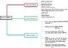 |
Figure 1 Different methods to solve CHPED problem. |
2 Literature review
For the CHPED problem, classical mathematical programming methods were presented in [2] and [3]. Dual, Partial-Separable programming was implemented in [2] in Fortran 77 language. Here, the CHP issue is divided into two levels involving the distribution of heat and power: the bottom level determines production levels based on provided multipliers, while the top level adapts these multipliers to ensure that power production matches the demand, the algorithm has slow convergence. In [3], A two-layered algorithm is proposed, and the CHP issue is divided into sub-problems related to the distribution of heat and power. The power dispatch problem is solved iteratively in the outer layer using the Lagrangian Relaxation approach. During each iteration, the inner layer solves the heat dispatch using the unit heat capacity provided by the outer layer. The two sub-problems are linked by the heat-power feasible operating region (FOR) limits of cogeneration units. However, the algorithm took a lot of time for each iteration. The direct solution was given to the CHPED problem in [4, 5]. In [4], the optimal marginal costs (λ − s) formula was utilized to compute the cost that corresponds to a given heat and power demand. In [5], an explicit formula has been created for calculating incremental costs for the ideal dispatch for the overall system. A study made in [6] offered a Linear Programming (LP) formulation with a unique structure and created a simplex algorithm that effectively makes use of this structure and is five times faster than simplex.
A deterministic network flow model using LP of a typical CHP system was made in [7], where a system λ − s matching the required power and heat demands formula was constructed. The Network flow model has the benefit of making it easier to interpret the data because it is simple to visualize the thermal and electric energy flows through the CHP equipment. The work of the Two-stage mathematical programming approach for the solution of the CHPED problem was done in [8]. An equivalent Mixed-Integer Quadratically Constrained Quadratic Program (MIQCQP) problem is resolved in the first stage. The solution region in the FOR is identified using the findings from solving Problem I. In [9], a microgrid with an EV charging station, CHP generation, renewable energy resource, external power grid, and natural gas station was developed, satisfying both electricity and heat energy demand. They have formulated a long-term cost minimization problem and proposed a Lyapunov optimization-based approach for real-time energy management. In [10], an optimal dispatch model for an Integrated Energy System (IES) based on carbon trading and CHP with Power to Gas (P2G) and Carbon Capture System (CCS) is proposed. In the research work [11], the Filled Function Method (FFM) was used to address the CHPED optimization problem. Furthermore, the Taguchi approach is integrated with the FFM and a developed TFFM to determine the optimal initial parameters. The most significant advantage of the TFFM is that it always produces the same result for identical inputs, and all solutions are within the feasible range.
A study in [12] described CHPED problems as a Markov decision process (MDP), which makes the model well encapsulated to maintain the input and output features of diverse devices. MDP provides a mathematical framework for simulating decision-making in which outcomes are partly dictated by chance and partly under the decision-maker’s control. This avoids complex linearization methods to manage non-smooth functions. An Enhanced Distributed Proximal Policy Optimization (EDPPO), which is an advanced deep reinforcement learning technique, is used to solve CHPED. In [13], a Deep Reinforcement Learning (DRL) based Crisscross Optimization (CSO) algorithm was mentioned. The purpose of adopting DRL is to decrease the number of dimensions and limit the range of the initial population in the CSO algorithm. Next, the Deep Deterministic Policy Gradient (DDPG) technique updated DRL by enabling quick decision-making to speed up CSO.
The method explained in [14] combined the Improved genetic algorithm and the multiplier updated in such a way that it has the advantage of automatically setting the randomly assigned penalty to the appropriate value and only needs a modest population size for the CHPED issue. In [15], the CHPED problem was solved with a self-adaptive real-coded GA by considering the equality and inequality constraints simultaneously while integrating a penalty parameter-less constraint management approach. To produce superior offspring, the distribution index in the Simulated Binary Crossover (SBX) operator is used to introduce population variety. This results in a population with a high degree of variety, which can both improve the likelihood of reaching the global optimum and delay premature convergence. Real-coded GA with improved Muhlenbein mutation (RCGA-IMM) [16] is used to address the CHPED issue while taking the effect of valve-point loading and transmission losses into account. The Muhlenbein mutation is implemented in basic RCGA for speeding up the convergence and improving the optimization problem results. Two new Collective Information (CI)-based techniques, CI-based particle search, and CI-based elite fine-tuning, were developed in Collective Information-Based PSO (CIBPSO) [17]. IBBMOPSO studied in [18] integrates four improved strategies, namely: (i) a non-linear adaptive particle updating strategy is presented to automatically tune the weights of the personal (pbest) and the global (gbest) best positions respectively, and to reduce the standard deviation for generating new particles; (ii) an improved strategy by comparing the sparsity of the pbest and target particle to update pbest; (iii) To get the gbest for each target particle, a modified strategy that chooses a random Pareto optimal solution from a newly filtered subset of the external archive is used, and (iv) a new approach that combines the slope and the crowding distance is used. To enhance global search capabilities and avoid convergence to local minima, the research in [19] proposed combining the Continuous-Greedy Randomized Adaptive Search Process (C-GRASP) with DE and developed the C-GRASP-DE algorithm. Two strategies – Gaussian-Cauchy mutation and parameter self-adaptation – are used in Self-Adaptive DE with Gaussian-Cauchy mutation (SDEGCM) to enhance performance in [20]. Moreover, SDEGCM employed a constraint repair technique to address complicated operational restrictions. The suggested SDEGCM has provided better values in terms of solution stability and accuracy for the large-scale CHPED problem. Opposition-based GSO is presented in [21] and used to solve the CHPED issue by considering factors like VPE, Transmission loss, etc. The GSO algorithm in [22] used opposition-based learning for both population initialization and intelligent iteration updating. The core ranging mechanism of the Modified-GSO (MGSO) was presented in [22] to solve the CHPED problem on a large-scale test systems and prevent premature convergence is known as the B-Spline Wavelet (BW) theory. A One-Rank Cuckoo Search Algorithm (ORCSA) approach was developed and utilized in [23] to achieve the best possible solution quality and computational efficiency. In [24], a Grey wolf optimization technique is used to reduce costs while taking valve point influences and the CHP units’ dual dependence on heat and electricity generation into account. The Harmony Search approach is integrated with GA and developed HSGA [25] to obtain the solution of the CHPED problem. This algorithm uses a unique crossover operator. Basically, HS is used to ensure a high probability of assessing the global optimum by identifying inferior individuals. In [26], an improved HS method for addressing the CHPED problem is provided, in which the bandwidth adjustment is updated to obtain better results in terms of operational cost. In [27], a swarm-based algorithm inspired by honeybee food foraging behaviour is applied to the CHPED problem. It was observed that the algorithm delivered a better solution with less computational work. An optimization method called the Invasive Weed Optimization (IWO) algorithm is employed to solve the CHPED issue, which is based on the ecological process of weed colonization and dissemination [28]. In [29], an integration of Opposition-Based Learning (OBL) with Teaching Learning Based Optimization (TLBO) was employed to solve the CHPED problem in order to achieve less computational time and lower operational costs. A hybrid Firefly and Self-Regulating PSO (FSRPSO) method is used in [30] to address the CHPED problem. The FSRPSO leveraged the strengths of both the Firefly Algorithm (FA) and the SRPSO processes to balance the exploration and exploitation phases. The appropriate convergence speed and accuracy of the Crisscross optimization algorithm are better due to the use of the two stated crossover operators [31]. The vertical crossover operator is changed in [32] while tackling large-scale CHPED optimization problems, considering VPE, power transmission losses, and POZs of conventional thermal units. In [33], the Multi-Verse Optimization (MVO) method was developed, and it makes use of three astrophysical concepts: white holes, black holes, and wormholes, which are used to explore the evolution of the cosmos. An improved marine predators’ optimization algorithm (IMPOA) was suggested in [34] for tackling the CHPED. In [35], a CSMO-Hybrid chameleon swarm algorithm and Mayfly optimization (MO) were proposed for tackling the CHPED issue that combines the Chameleon Swarm Algorithm (CSA) and MO. In [36], a powerful algorithm was designed by combining the Modified Grasshopper Optimization Algorithm (MGOA) and the improved Harris Hawks Optimizer (IHHO) in order to achieve a better balance between the early phases of global search and the latter stages of global convergence. MGOA-IHHO is the abbreviation for the proposed endeavor. The CHPED issue was investigated by combining a Strong Exploitation Strategy (SES) with a social network search (SNS) optimizer to produce an Improved SNS (ISNS) in [37] that improved SNS performance by boosting searching around the best view of all users. A metaheuristic method, Imperialist Competitive Harris Hawks Optimization [38], is used to address the Multi-Zone CHPED (MZCHPED) problem.
The application of classical methods is limited to solving CHPED issues under certain simplifying assumptions, which serve to make the optimization problem more manageable and less complex. Within deterministic models, it is assumed that the problem is free from both inherent and external disruptions and inaccuracies. This ideal assumption is invalid in practical implementations, and the differences can be significant under certain circumstances. Deep learning methods need improvement to be applicable to complex CHPED problems. Stochastic models are more commonly used for analyzing power dispatch problems because they can account for the presence of imprecise and unpredictable components that are typically present in system operation. Currently, numerous optimization methods that simulate different natural phenomena have been suggested and utilized to address this intricate challenge. These algorithms assert that they outperform similar optimization algorithms in terms of precision and execution time. According to the No Free Lunch Theorem [39], there is no metaheuristic strategy that guarantees the global optimal solution for the CHPED problem. Therefore, to further optimize costs within a reasonable execution time, a new algorithm was developed and used in the current research.
The main contributions of this paper are summarised as follows:
-
For the first time, a novel bio-inspired method called the LCA is introduced to address the medium and large-scale CHPED problems.
-
Random Opposition-Based Learning (ROBL) strategy is used to initialize the population. This strategy accelerates the search process and avoids getting stuck in a local optimum.
-
Valve-point loading effect is considered for power-only units.
-
The proposed method has been proven through extensive trials for solving the CHPED problem on four test systems, demonstrating its efficacy, efficiency, and superiority.
3 Problem formulation
A CHP system comprises power-only units that specifically generate electrical power, CHP units that concurrently generate power and heat, and heat-only units that generate heat specifically. This study aims to identify the most favourable outcomes while taking into account the limitations imposed by electricity consumption, power demand, heat demand, and other relevant factors.
The general optimization problem can be formulated as follows: (1)
(1)
 (2)
(2)
 (3)where, “f” is an objective function to be minimized. g(x, u) represents the nonlinear equality constraints, such as real power and heat constraints. h(x, u) represents the inequality constraints of the functional operating constraints, such as the Power limits of power-only units, the heat limits of heat-only units, and the feasible operating region of CHP units.
3.1. Objective Function:
Minimization of generation cost of CHP system: The aim of the CHP economic dispatch problem is to minimize the Cost of fuel, and is expressed as: (4)where C is the cost of overall production. Ppi is the power output, where pi is the power of ith power-only unit with valve point loading effect. Pchpj is the power output and Tchpj is the heat output, where chpj is the jth CHP unit. Thk is the heat output, where hk is the kth heat-only unit. Cpi, Cchpj, and Chk are the unit costs when the output is Ppi, Pchpj, Tchpj, and Thk, respectively Cpi, Cchpj, and Chk are defined below:
 (5)
(5)
Typically, the fuel cost function for thermal power production units is represented by a quadratic function of active power outputs. Large power-producing units with steam turbines feature several steam admission valves. To obtain a continuously growing power output, these valves are opened one after the other. The valve opening results in throttling losses and wire pulling, which abruptly raises the heat rate. The presence of multiple valves in large steam turbine generators causes a phenomenon called the valve-point loading effect, which results in a rippling effect on the input-output characteristic [40]. The valve-point loading effect has been represented here by adding a sinusoidal term to the conventional cost function [41] and expressed in equation (5). Therefore, the output of the generation unit is not consistently stable, as depicted in Figure 2. Hence, the objective function is nonconvex. The cost functions of CHP units and heat-only units are expressed as follows: (6)
(6)
 (7)where ai, bi, ci, di, and ei are the cost coefficients of the ith power-only unit.
  is the minimum limit of the ith power-only unit. αj, β j, γj, δj, εj, and ζj are the cost coefficients of the jth CHP unit. φk, ηk, and λk are the cost coefficients of the kth heat-only unit.
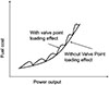 |
Figure 2 Cost curve of power units. |
3.2 Constraints
3.2.1 Equality constraints
The power and heat outputs must satisfy the corresponding demands for electricity and heat.
 (8)
(8)
 (9)where PD and TD are the power demand and heat demand, respectively.
3.2.2 Inequality constraints
(a) Inequality constraints of power-only unit
The upper and lower bounds of the power-only unit’s output can be represented as follows: (10)where
  and
and  are the lower and higher outputs of ith power-only unit, respectively.
(b) Inequality constraints of heat-only unit
The upper and lower bounds of the Heat-only unit’s output can be represented as follows: (11)where
  and
and  are the maximum and minimum outputs of k
th heat-only unit, respectively.
are the maximum and minimum outputs of k
th heat-only unit, respectively.
(c) Inequality constraints of the CHP unit
Power and heat generated by CHP units should be within the limits defined by the feasible operating region (FOR), as shown in Figure 3. (12)
(12)
 (13)
(13)
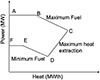 |
Figure 3 Feasible operating region of cogeneration plants. |
FOR is limited by (a) the generator’s capacity-based maximum and minimum power output, which is the upper limit for overloading risks and the lower limit for unstable operation; (b) the maximum and lower heat outputs, where low heat output indicates fuel waste and high heat output indicates exceeding design limits; and the addition of heat exchangers unit design, which limits the heat. (c) Since all steam is used for heating after power generation, the backpressure line for the CHP unit’s steam turbine specifies the high heat or low power limit; (d) the condensing line, which is important to the condensing turbine and is led by maximum power output, but reduces useful heat. (e) Iso-fuel curves, for constant fuel input.
4 Methodology to solve the CHPED problem by using the Liver Cancer algorithm
LCA is a novel biologically inspired technique introduced by Essam H. Houssein et al. in 2023 [42]. The behaviour of liver tumors serves as a source of inspiration for LCA and incorporates biological concepts into its optimization process. This makes it a unique and practical method for selecting features. Ten global optimization problems from the CEC’2020 test suite have been employed to evaluate the proposed LCA against several optimization algorithms, and from the results, it is concluded that the LCA has given better results in comparison to the other algorithms.
4.1 Liver cancer algorithm
The LCA algorithm is specifically developed to replicate the growth and dissemination patterns of liver tumors, which are cancerous growths in the liver that can significantly impair the body’s functioning. The intricate nature of liver tumor growth, which involves interactions with the milieu and signalling pathways such as angiogenesis, immune evasion, and genetic alterations, serves as the motivation for the creation of LCA. Regarding optimization, the LCA algorithm imitates the pattern of expansion and dissemination of liver tumors within the liver. The algorithm’s design is influenced by the adaptive nature of tumors, as they seek the most conducive environment for growth within the liver, as shown in Figure 4. The LCA technique comprises multiple steps, each characterized by unique mathematical formulations, to accurately simulate the growth and behaviour of the tumour. The LCA algorithm uses ROBL to initialize the population. LCA employs variable approaches such as the jump strength method, Levy’s flight function, and genetic operators during the exploitation phase, and this algorithm thoroughly explores the search space while striking a balance between local and global searches. The mutation rate is changed based on the number of iterations, and a higher mutation rate allows for the investigation of interesting new places while also preventing the algorithm from becoming stranded at a local minimum. As a result, a more optimal value can be obtained in less time. These features of LCA mentioned above make the LCA better than other contemporary algorithms mentioned in this work.
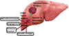 |
Figure 4 Tumor spread in liver. |
4.1.1 Tumor size calculation
The LCA algorithm [42] relies on the estimation of the tumor’s size, which is crucial for the succeeding steps. A mathematical model was utilized to assess the size of the tumor. This model is based on the assumption that tumors have a hemi-ellipsoid shape, as shown in Figure 5, which has been found in other types of malignancies, including liver cancer [43]. The tumor is characterized by three dimensions: width, length, and height. Nevertheless, directly measuring the height dimension poses difficulties and is approximated via a mathematical model.
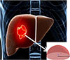 |
Figure 5 Shape of tumor. |
The size and position of the first tumor are determined using equation (14), which uses ROBL to create a starting population with a wide range of search exploration abilities.
 (14)where i = 1, 2, … N and j = 1, 2, … D. lb and ub represent the lower and upper boundaries of the decision variables, respectively. D is the dimension of the search area. The current position is Positioni, and the opposite position is
  . rd is a random number between 0 and 1. This random number is used to establish the initial population. The tumor position’s size is determined by calculating the length of its diameters, which include width, height, and length, as shown in equation (15). The values for width and height are randomly generated numbers between 0 and 1.
 (15)where f, a constant equal to 1 for a specific type of tumor [44].
4.1.2 Tumor replication
The updating of tumor location is made based on different stages of cancer. The stage is defined by tumor position and size.
Stage I: If the tumor size is small, the tumor location is updated by the perch based on other family members or on a random tall tree. The increase in tumor position size (position) is calculated by equation (15).
Stage II: If the tumor size is increased and pushed to surrounding tissues, the tumor location is updated by the random jump strength of the tumor (Y) as shown in equation (17). Tumors replicate themselves in another place in the same liver organ in this stage.![Mathematical equation: $$ {\left({PG}\right)}^i=\frac{\mathrm{d}V}{\mathrm{d}t}={r*}\enspace \mathrm{Position}\enspace t\in \left[1\dots T\right]\hspace{1em}\mathrm{and}\hspace{1em}\enspace i\in \left[1\dots N\right], $$](/articles/stet/full_html/2026/01/stet20240122/stet20240122-eq23.gif) (16)
(16)
 (17)
(17)
Stage III: If the tumor size is increased or multiple tumors are formed regionally, the tumor location is updated by the best way out of two methods: 1. Jump strength (Y), and 2. Based on Levy’s flight function (Z) as shown in equation (22), this gives the best dive into the liver portions to capture them in competitive situations. Spread is increased to obtain a location where control of spread is minimal.
 (18)where S is a random number between 0 and 1,
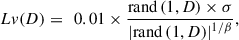 (19)where D is the dimension of variables to be generated,
![Mathematical equation: $$ {\sigma =\left[\left(\frac{\mathrm{\Gamma }\left(1+\mathrm{\beta }\right)\mathrm{\enspace }\times \mathrm{\enspace sin}(\frac{{\pi \beta }}{2})}{\mathrm{\Gamma }\left(\frac{1+\mathrm{\beta }}{2}\right)\times \beta \times {(2)}^{\left(\frac{\beta -1}{2}\right)}}\right)\right]}^{1/\beta }, $$](/articles/stet/full_html/2026/01/stet20240122/stet20240122-eq27.gif) (20)where β = 1.5 and
(20)where β = 1.5 and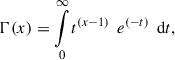 (21)
(21)
 (22)
(22)
4.1.3 Tumor spreading using crossover and mutation
The final phase of the LCA algorithm signifies the advancement of a tumor to metastatic liver cancer, a sophisticated manifestation of the illness that originates in the liver but disseminates to additional regions of the body [45]. The LCA algorithm utilizes genetic operators, such as mutation and crossover, to provide extra variety in order to achieve its objective.
Stage IV: If the tumor size is spread to other organs, the tumor location is updated by a genetic algorithm that picks the best of three ways: mutated Y, mutated Z, and Crossover as shown in equation (27). (23)
(23)
 (24)
(24)
 (25)
(25)
![Mathematical equation: $$ {W}_{\mathrm{cross}}^{\enspace }=\mathrm{\tau }\enspace \mathrm{*}\enspace {y}_{\mathrm{Mut}}+\left(1\enspace -\enspace {\mathrm{\tau }}^\mathrm{\prime}\right)\mathrm{*}{z}_{\mathrm{Mut}},\hspace{1em}\enspace {\tau }\enspace \ne \enspace {\tau }\enspace {\prime}\enspace \mathrm{random}\enspace \mathrm{values}\enspace [\mathrm{0,1}] $$](/articles/stet/full_html/2026/01/stet20240122/stet20240122-eq33.gif) (26)
(26)
 (27)
(27)
Pseudocode of Liver Cancer algorithm
1: Initialization: Initialize the population of liver tumor positions/locations by equation (14).
2: while (The termination requirement has not been satisfied) do
3: Estimate the tumor position fitness value. ⊳ Exploitation phase
4: if (Position < limit1), then
5: Update the tumor position with equation (15)
6: end if
7: else if (Position >= limit1) and (Position < limit2)
8: Update the tumor position by equation (17)
9: else if (Position >= limit2) and (Position < limit3)
10: Using equation (22), modify the position replication of the current search agent.
11: else Apply genetic operator equations (23)–(26) to calculate Position tumor spreading.
12: Using equation (27), update the current search agent’s tumor position replication.
13: Validate and adjust the tumor positions to satisfy the constraints
13: Compute each tumor position fitness and search for best. ⊳ Exploration phase
14: t = t + 1
15: end while
16: Return best Fitness, Position
4.2 LCA in CHPED
N is the population size. Number of dimensions D that depicts Tumor location elements is l1 + lc1 + lh1, where l1 = Np−1, lc1 = Nc, lh1 = Nh−1, excluding slack power and slack heat units for power-only and heat-only units, respectively. The initialization of the population for X is given as equation (28).![Mathematical equation: $$ X=\left[\begin{array}{c}{X}_{\enspace }^1\\.\\.\\.\\ \enspace {X}_{\enspace }^i\\.\\.\\.\\.\\ {X}_{\enspace }^N\end{array}\right]=\left[\begin{array}{ccc}\begin{array}{c}{X}_1^1,\enspace.\enspace.\enspace.\enspace {X}_{{Np}-1}^1,.\enspace.\enspace.\\.\\.\\.\\ {X}_1^i,\enspace.\enspace.\enspace.\enspace {X}_{{Np}-1}^i,.\enspace.\enspace.\\.\\.\\.\\.\\ {X}_1^N,\enspace.\enspace.\enspace.\enspace {X}_{{Np}-1}^N,.\enspace.\enspace.\end{array}& \begin{array}{c}{X}_{{Np}-1+{Nc}}^1,.\enspace.\enspace.\\ \\ \\ \\ {X}_{{Np}-1+{Nc}}^i,.\enspace.\enspace.\\ \\ \\ \\ \\ {X}_{{Np}-1+{Nc}}^N,.\enspace.\enspace.\end{array}& \begin{array}{c}{X}_{{Np}-1+{Nc}+{Nh}-1}^1\\.\\.\\.\\ {X}_{{Np}-1+{Nc}+{Nh}-1}^i\\.\\.\\.\\.\\ {X}_{{Np}-1+{Nc}+{Nh}-1}^N\end{array}\end{array}\right]. $$](/articles/stet/full_html/2026/01/stet20240122/stet20240122-eq35.gif) (28)
(28)
The initial population is initialized using the ROBL technique (first generation data), satisfying inequality constraints of power-only units, heat-only units, and Cogeneration units. Fitness values, C for economic dispatch, are calculated using equation (4). The initial population of tumor location includes Np − 1 power-only units, Nh − 1 heat-only units, Nc cogeneration plants, and excludes the slack power-only unit and the slack heat-only unit.
4.2.1 Constraints handling mechanism
The initialized population is populated in such a manner that it meets the inequality constraints of all Power-only except slack power-only unit, all Heat-only plants except for the slack heat-only unit, and all CHP plants. Slack power and slack heat are calculated to fulfill the power and heat demands using equations (29) and (30). Thus, equality and inequality constraints are met except for the inequality constraints of the slack power-only unit and the slack heat-only unit. The values of slack power and slack heat obtained are validated for capacity limits. (29)
(29)
 (30)
(30)
 (31)
(31)
 (32)
(32)
 (33)
(33)
 (34)
(34)
If they do not satisfy inequality constraints, penalty for power and penalty for heat are calculated by taking a very large penalty factor [46, 47] accordingly, as shown in equations (31)–(34). The total penalty is the sum of the power penalty and the heat penalty. Penalty is included in the objective function C. The LCA Algorithm will try to minimize the objective function C, and this can occur when the penalty is zero.
In each iteration, the best of fitness values (local best) calculated so far is assigned to Tumor Energy, and the corresponding data is assigned to Tumor location. In each iteration, the tumor size is calculated. Depending on tumor size (stage of Liver Cancer), next-generation data is updated one by one in the population. The fitness value of the next generation is calculated. If this value is less than the earlier (local best) value, then the Fitness value is assigned to Tumor Energy, and that data is assigned to Tumor location. This is looped until the total number of iterations is reached, as shown in the flow chart.
4.2.2 Flow chart
The flow chart is showcased in Figure 6.
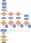 |
Figure 6 Flow chart of LCA applied to solve CHPED problem. |
4.3 Simulation results and discussion
In order to showcase the efficiency and resilience of the suggested algorithm, it is applied to CHP systems with 48 units, 96 units, and 192 units. The simulation programs were implemented on a PC having Intel Core i5, 3.20 GHz, and 16GB RAM in MATLAB 2013a environment. All three test cases include the valve point loading effects for the power-only units. The LCA algorithm is run for 200 iterations with a population size of 60 for all the test cases. The parameter limits are 0.8 and 1.96 as indicated in [42]. After executing the program for a number of trials using different values for the parameters, it is observed that the parameter values shown in Table 1 are the best possible values that yielded better results. Hence, the parameters are set to the values shown in Table 1.
The parameter setting of the proposed method.
4.3.1 Testcase 1
In testcase 1, there are 26 power-only units, 12 CHP units, and 10 heat-only units, so the total units is 48. The data taken from [48] for the 48-unit system is shown in Table 2. The power limits for all power-only units, heat limits for all heat-only units, and the feasible operating region (FOR) for all CHP units are mentioned in Table 2. Units from P1 to P26 are 26 power-only units. Units from C1 to C12 are 12 CHP units. Units from H1 to H10 are 10 heat-only units. The power demand is 4700 MW, and the heat demand is 2500 MWth. To find the optimal performance of the LCA algorithm, the parameters are set to the values shown in Table 1. The convergence curve of case 48 using LCA is shown in Figure 7. From this figure, it is observed that the value of the penalty is zero from the first iteration onwards, and this depicts the efficiency of the algorithm in populating the values satisfying the constraints. Radar charts shown in Figures 8 and 9 support validating that the powers and heats generated by all the units satisfy the inequality constraints. The orange, blue, and red color charts in Figures 8 and 9 indicate the maximum, minimum, and actual values of all 26 power-only units and 10 heat-only units, respectively. From these figures, it is clear that the powers and heats generated are within the minimum and maximum limits for all power-only and heat-only units. To verify the satisfaction of constraints for the CHP system, line charts are utilized. Figures 10a–10d verify if the generations of cogeneration plants are within the feasible operating regions. C1 (HC1, PC1) is a point referring to the cogeneration plant C1 that generates heat HC1 and power PC1. All 12 cogeneration plants are highlighted in Figures 10a–10d. It can be seen that all cogeneration plants generate power and heat within FORs. Hence, all the inequality constraints are satisfied. For verification of power equality constraints, the powers generated by all power-only units and CHP units were added, and the result obtained was 4700 MW, which is the same as the total power demand. In similar lines, for the heat equality constraint, the heat produced by all CHP units and all heat-only units was added, and the sum obtained was 2500 MWth, which satisfies the heat demand. Hence, equality restrictions are also satisfied. The results for testcase 1 obtained by the LCA are compared with TVAC-PSO, OTLBO, TVAC-GSA-PSO, SDEGCM, DRL-CSO, and FSRPSO and are exhibited in Table 3. It is shown that the LCA technique gives the minimum best cost for case 48 of 113,616.5734 $/h (Dollar per hour) as compared to other techniques. The proposed LCA demonstrates convergence to the optimal value, ensuring the efficiency and reliability of the recommended technique, and achieves a superior solution of higher quality within reasonably fewer iterations when compared to the other algorithms mentioned.
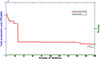 |
Figure 7 Convergence curve using LCA for Testcase 1. |
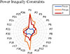 |
Figure 8 Power outputs of testcase 1. |
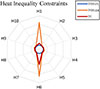 |
Figure 9 Heat outputs of testcase 1. |
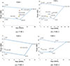 |
Figure 10 (a): FOR 1. (b): FOR 2; (c) FOR 3; (d) FOR 4. |
Cost function of all units of Testcase 1.
Comparison of LCA with other algorithms for Testcase 1.
4.3.2 Testcase 2
To verify the effectiveness of the proposed algorithm, it is implemented and tested for a larger-scale 96-unit CHP system. In 96-unit CHP system, there are 52 power-only units, 24 CHP units, and 20 heat-only units. Test data for 96 units is indicated in [51]. Units from P1 to P52 are 52 power-only units. Units from C1 to C24 are 24 CHP units. Units from H1 to H20 are 20 heat-only units. The power demand is 9400 MW, and the heat demand is 5000 MWth. To observe the better performance of the LCA algorithm, the parameters are set to the values shown in Table 1. The orange, blue, and red colors in Figures 11 and 12 indicate the maximum, minimum, and actual values of the powers and heats generated. Radar charts clearly show that the powers and heats generated are within the minimum and maximum limits for all power-only and heat-only units. All 24 cogeneration plants are highlighted in Figures 13a–13d. It can be seen that all the cogeneration plants generate power and heat within FORs. Hence, all the inequality constraints are met for testcase 2. Equality constraints are also satisfied. The details of the results using LCA are shown in Table 4. Comparison of the results of the best cost of the proposed algorithm is made with other algorithms like CSO, ISNS, SADEGCM, IMPOA, and DRL-CSO in Table 5. It can be seen that the proposed algorithm outperforms all other algorithms for testcase 2. The minimum cost of LCA is 220,107.797 $/h, whereas the other algorithms are in the range of 233,326.532 $/h. Nearly 13000 $/h amount is saved using the proposed algorithm LCA. It is evident that the LCA is a more effective algorithm in solving CHPED problems.
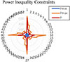 |
Figure 11 Power outputs of testcase 2. |
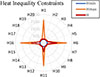 |
Figure 12 Heat outputs of testcase 2. |
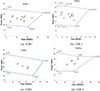 |
Figure 13 (a) FOR1; (b) FOR 2; (c) FOR3; (d) FOR 4. |
Power and heat outputs for Testcase 2 by using LCA.
Comparison of LCA with other methods for Testcase 2.
4.3.3 Testcase 3
Furthermore, to test the performance of the proposed algorithm LCA for very large scale, it is implemented for 192 units testcase 3. Testcase 3 includes 104 power-only units, 48 cogeneration units, and 20 heat-only units. Test data for 192 units is available in [13, 52, 53]. Units from P1 to P104 are 104 power-only units. Units from C1 to C48 are 48 number of CHP units. Units from H1 to H40 are 40 heat-only units. The power demand is 18,800 MW, and the heat demand is 10,000 MWth. To obtain a better performance of the LCA algorithm, the parameters are set to the values shown in Table 1. All the equality and inequality restrictions are met for testcase 3. The details of the results using LCA are shown in Table 6. The values of power are in MW and the heat in MWth. In Table 7, the results are compared to other methods such as CSO, NDIDE, HNTMACSO, and DRL-CSO. It is visible clearly that the LCA algorithm yields better results compared to others.
Power and heat outputs for Testcase 3 by using LCA.
Comparison of LCA with other methods for Testcase 3.
4.4 Statistical analysis of the performance of the Liver Cancer Algorithm
The statistical values described by minimum, maximum, average values, and standard deviation, along with the execution time obtained from 20 trials of different algorithms, including LCA for testcases 1, 2, and 3, are shown in Table 8. The execution time of LCA is less than that of TVAC-PSO, SDEGCM, DRL-CSO, and OTLBO algorithms for testcase 1. The costs are significantly less compared to all other algorithms for all the test cases taken in this paper.
Performance of LCA compared to other methods.
It is also observed that the proposed algorithm gives the same optimal value most of the time when executed consecutively. The minimum value is obtained in nearly 80% of 20 trials for testcase 48 using LCA, as shown in Figure 14. Also, to appreciate the performance of the proposed algorithm, the Wilcoxon signed rank test is carried out. This test is conducted at a significance level of 0.05, denoted as α. Statistical analysis provides the information regarding the acceptance or rejection of any hypothesis. Hypotheses can be evaluated by comparing statistical data with significance analysis, which determines whether to reject or retain them. If the statistical value is below the significance level, the hypothesis H1 will be accepted; otherwise, it will be rejected. This indicates that the algorithm could minimize the cost to a greater extent, satisfying all the constraints. Table 9 displays the preservation of the hypothesis by the utilisation of the Wilcoxon signed-rank test.
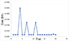 |
Figure 14 Best costs obtained in 20 trials of LCA. |
Wilcoxon signed rank test.
Conclusion
This article presents a novel bio-inspired LCA as a demonstration of its effectiveness in addressing the CHPED problem for medium and large-scale systems. The proposed optimization methodology utilized a strong exploitative strategy, ROBL, to initialize the population, where searching is done throughout the search space and applied Levy’s flight function, genetic operators to update the population in one iteration, and a precise exploration technique for searching the best solution. This approach generated optimum solutions for the objective function and enhanced the convergence rate of the algorithm. In order to assess the superiority of the bio-inspired LCA, 3 test systems were employed, where one is a 48-unit medium test system and two large-scale test systems, 96 and 192 units, are employed, considering valve point impacts for all power-only units. The applications underwent testing and implementation under power and heat-loading conditions. To assess the efficacy of the LCA technique, a comparison was conducted using recently developed algorithms. The simulation results indicate that the proposed LCA technique surpasses other algorithms in terms of performance. The simulation results of the LCA demonstrate that the proposed algorithm’s performance remains unaffected by various nonlinearities resulting from valve point loading of thermal units, as well as the size of the system. This indicates the algorithm’s robustness. The proposed strategy has the potential to enhance the rate of convergence and provide a solution that encompasses the whole problem space. Consequently, LCA has been successfully utilized to investigate CHPED concerns. From statistical analysis, it can be concluded that LCA exerts an excellent compromise between execution time and generation costs. The generation cost is reduced, and the time of execution is also less. It is also observed that the proposed algorithm consistently gives the best value. In future work, the use of the proposed algorithm may be implemented to solve the multiobjective CHP economic emission dispatch problem, including renewable energy sources.
References
- Gowrishankar V., Angelides C., Druckenmiller H. (2013). Combined heat and power systems: Improving the energy efficiency of our manufacturing plants, buildings, and other facilities. NRDC Issue Paper 13-04-B. Available at https://www.nrdc.org/sites/default/files/combined-heat-power-IP.pdf. [Google Scholar]
- Guo T., Henwood M.I., Van Ooijen M. (1996) An algorithm for combined heat and power economic dispatch. IEEE Trans. Power Syst. 11, 1778–1784. [Google Scholar]
- Rooijers F.J., Van Amerongen R.A. (1994) Static economic dispatch for co-generation systems, IEEE Trans. Power Syst. 9, 1392–1398. [Google Scholar]
- Rao P.S.N. (2006) Combined heat and power economic dispatch: A direct solution, Electr. Power Compo. Syst. 34, 9, 1043–1056. https://doi.org/10.1080/15325000600596775. [Google Scholar]
- Ohaegbuchi D.N., Maliki O.S., Okwaraoka C.P.A., Okwudiri H.E. (2022) Solution of combined heat and power economic dispatch problem using direct optimization algorithm, Energy Power Eng. 14, 737–746. https://doi.org/10.4236/epe.2022.1412040. [Google Scholar]
- Lahdelma R., Hakonen H. (2003) An efficient linear programming algorithm for combined heat and power production, Eur. J. Oper. Res. 148, 1, 141–151. https://doi.org/10.1016/s0377-2217(02)00460-5. [Google Scholar]
- Cho H., Luck R., Eksioglu S.D., Chamra L.M. (2009) Cost-optimized real-time operation of CHP systems, Energy Build. 41, 4, 445–451. https://doi.org/10.1016/j.enbuild.2008.11.011. [Google Scholar]
- Moradi Dalvand M., Nazari Heris M., Mohammadi Ivatloo B., Galavani S., Rabiee A. (2019) A two-stage mathematical programming approach for the solution of combined heat and power economic dispatch, IEEE Syst. J. 14, 2, 2873–2881. https://doi.org/10.1109/JSYST.2019.2909627. [Google Scholar]
- Shen Z., Wu C., Wang L., Zhang G. (2021) Real-time energy management for microgrid with EV station and CHP generation, IEEE Trans. Netw. Sci. Eng. 8, 2, 1492–1501. https://doi.org/10.1109/tnse.2021.3062846. [Google Scholar]
- Jour M.Y., Wang H., Hong F., Yang J., Chen Z., Cui H., Feng J. (2021) Modeling and optimization of combined heat and power with power-to-gas and carbon capture system in integrated energy system, Energy 236, 121392. https://doi.org/10.1016/j.energy.2021.121392. [Google Scholar]
- Eke İ. (2022) Combined heat and power economic dispatch by Taguchi-based filled function, Eng. Optim. 55, 5, 791–805. https://doi.org/10.1080/0305215X.2022.2034802. [Google Scholar]
- Zhou S., Hu Z., Gu W., Jiang M., Chen M., Hong Q., Booth C. (2020) Combined heat and power system intelligent economic dispatch: A deep reinforcement learning approach, Int. J. Electr. Power Energy Syst. 120, 106016. https://doi.org/10.1016/j.ijepes.2020.106016. [Google Scholar]
- Meng A., Rong J., Yin H., Luo J., Tang Y., Zhang H., Li C., Zhu J., Yin Y., Li H., Liu J. (2024) Solving large-scale combined heat and power economic dispatch problems by using deep reinforcement learning based crisscross optimization algorithm, Appl. Therm. Eng. 245, 122781. https://doi.org/10.1016/j.applthermaleng.2024.122781. [Google Scholar]
- Su C.T., Chiang C.L. (2004) An incorporated algorithm for combined heat and power economic dispatch, Electr. Power Syst. Res. 69, 187–195. [Google Scholar]
- Subbaraj P., Rengaraj R., Salivahanan S. (2009) Enhancement of combined heat and power economic dispatch using self-adaptive real-coded genetic algorithm, Appl. Energy 86, 915–921. [Google Scholar]
- Haghrah A., Nazari-Heris M., Mohammadi-Ivatloo B. (2016) Solving combined heat and power economic dispatch problem using real-coded genetic algorithm with improved Mühlenbein mutation, Appl. Therm. Eng. 99, 465–475. [Google Scholar]
- Chen X., Li K. (2022) Collective information-based particle swarm optimization for multi-fuel CHP economic dispatch problem, Knowledge-Based Syst. 248, 108902. [Google Scholar]
- Xiong G., Shuai M., Hu X. (2022) Combined heat and power economic emission dispatch using improved bare-bone multi-objective particle swarm optimization, Energy 244-B, 123108. [Google Scholar]
- Neto J.X.V., Reynoso-Meza G., Ruppel T.H., Mariani V.C., dos Santos Coelho, L. (2017) Solving non-smooth economic dispatch by a new combination of continuous GRASP algorithm and differential evolution, Int. J. Electr. Power Energy Syst. 84, 13–24. [Google Scholar]
- Chen X., Shen A. (2022) Self-adaptive differential evolution with Gaussian–Cauchy mutation for large-scale CHP economic dispatch problem, Neural Comput. Appl. 34, 11769–11787. https://doi.org/10.1007/s00521-022-07068-w. [CrossRef] [Google Scholar]
- Basu M. (2015) Combined heat and power economic dispatch using opposition-based group search optimization, Int. J. Electr. Power Energy Syst. 73, 819–829. [Google Scholar]
- Davoodi E., Zare K., Babaei E. (2017) A GSO-based algorithm for combined heat and power dispatch problem with modified scrounger and ranger operators, Appl. Therm. Eng. 120, 36–48. [Google Scholar]
- Nguyen T.T., Vo D.N. (2015) The application of one rank cuckoo search algorithm for solving economic load dispatch problems, Appl. Soft Comput. 37, 763–773. https://doi.org/10.1016/j.asoc.2015.09.010. [Google Scholar]
- Jayakumar N., Subramanian S., Ganesan S., Elanchezhian E. (2015) Combined heat and power dispatch by grey wolf optimization. Int. J. Energy Sector Manage. 9, 523–546. [Google Scholar]
- Huang S.H., Lin P.C. (2013) A harmony-genetic based heuristic approach toward economic dispatching combined heat and power, Int. J. Electr. Power Energy Syst. 53, 482–487. [Google Scholar]
- Khorram E., Jaberipour M. (2011) Harmony search algorithm for solving combined heat and power economic dispatch problems, Energy Convers. Manage. 52, 1550–1554. [Google Scholar]
- Basu M. (2011) Bee colony optimization for combined heat and power economic dispatch, Expert Syst. Appl. 38, 13527–13531. [Google Scholar]
- Jayabarathi T., Yazdani A., Ramesh V., Raghunathan T. (2014) Combined heat and power economic dispatch problem using the invasive weed optimization algorithm, Front. Energy 8, 25–30. [Google Scholar]
- Roy P.K., Paul C., Sultana S. (2014) Oppositional teaching learning-based optimization approach for combined heat and power dispatch, Int. J. Electr. Power Energy Syst. 57, 392–403. [Google Scholar]
- Nasir M., Sadollah A., Aydilek İ.B., Lashkar Ara A., Nabavi-Niaki S.A. (2021) A combination of FA and SRPSO algorithm for combined heat and power economic dispatch, Appl. Soft Comput. 102, 107088. https://doi.org/10.1016/j.asoc.2021.107088. [Google Scholar]
- Meng A.-B., Chen Y.-C., Yin H., Chen S.-Z. (2014) Crisscross optimization algorithm and its application, Knowledge-Based Syst. 67, 218–229. [Google Scholar]
- Meng A., Mei P., Yin H., Peng X., Guo Z. (2015) Crisscross optimization algorithm for solving combined heat and power economic dispatch problem, Energy Convers. Manage. 105, 1303–1317. https://doi.org/10.1016/j.enconman.2015.09.003. [Google Scholar]
- Mirjalili S., Mirjalili S.M., Hatamlou A. (2016) Multi-verse optimizer: A nature-inspired algorithm for global optimization, Neural Comput. Appl. 27, 495–513. https://doi.org/10.1007/s00521-015-1870-7. [Google Scholar]
- Shaheen A.M., Elsayed A.M., Ginidi A.R., El-Sehiemy R.A., Alharthi M.M., Ghoneim S.S.M. (2022) A novel improved marine predators algorithm for combined heat and power economic dispatch problem, Alex. Eng. J. 61, 3, 1834–1851. https://doi.org/10.1016/j.aej.2021.07.001. [CrossRef] [Google Scholar]
- Rizk-Allah R.M., Hassanien A.E., Snasel V. (2022) A hybrid chameleon swarm algorithm with superiority of feasible solutions for optimal combined heat and power economic dispatch problem, Energy 254, 124340. https://doi.org/10.1016/j.energy.2022.124340. [Google Scholar]
- Ramachandran M., Mirjalili S., Nazari-Heris M., Parvathysankar D.S., Sundaram A., Gnanakkan C.A.R. (2022) A hybrid grasshopper optimization algorithm and Harris Hawks optimizer for combined heat and power economic dispatch problem, Eng. Appl. Artif. Intell. 111, 104753. https://doi.org/10.1016/j.engappai.2022.104753. [Google Scholar]
- Gafar M., Ginidi A., El-Sehiemy R., Sarhan S. (2022) Improved SNS algorithm with high exploitative strategy for dynamic combined heat and power dispatch in co-generation systems, Energy Rep. 8, 8857–8873. https://doi.org/10.1016/j.egyr.2022.06.054. [Google Scholar]
- Nazari A., Abdi H. (2022) Solving the combined heat and power economic dispatch problem in multi-zone systems by applying the imperialist competitive Harris hawks optimization, Appl. Soft Comput. 26, 12461–12479. https://doi.org/10.1007/s00500-022-07159-9. [Google Scholar]
- Wolpert D.H., Macready W.G. (1997) No free lunch theorems for optimization, IEEE Trans. Evol. Comput. 1, 1, 67–82. https://doi.org/10.1109/4235.585893. [CrossRef] [Google Scholar]
- Decker G.L., Brooks A.D. (1958) Valve point loading of turbines, Trans. Am. Inst. Electr. Eng. Power Apparatus Syst. 77, 481–484. [Google Scholar]
- Pulluri H., Kumar N.G., Rao U.M., Preeti, Kumar M.G. (2019) Krill herd algorithm for solution of economic dispatch with valve-point loading effect, in: Applications of computing, automation and wireless systems in electrical engineering, Vol. 553, Springer, pp. 431–440. https://doi.org/10.1007/978-981-13-6772-4_33. [Google Scholar]
- Houssein E.H., Oliva D., Abdel Samee N., Mahmoud N.F., Emam M.M. (2023) Liver Cancer Algorithm: A novel bio-inspired optimizer, Comput. Biol. Med. 165, 107389. https://doi.org/10.1016/j.compbiomed.2023.107389. [Google Scholar]
- Feldman J.P., Goldwasser R., Mark S., Schwartz J., Orion I. (2009) A mathematical model for tumor volume evaluation using two-dimensions, J. Appl. Quant. Methods 4, 4, 455–462. [Google Scholar]
- Sápi J., Kovács L., Drexler D.A., Kocsis P., Gajári D., Sápi Z. (2015) Tumor volume estimation and quasi-continuous administration for most effective bevacizumab therapy, PLoS One 10, 11, e0142190. [Google Scholar]
- Vatandoust S., Price T.J., Karapetis C.S. (2015) Colorectal cancer: Metastases to a single organ, World J. Gastroenterol. 21, 41, 11767. https://doi.org/10.3748/wjg.v21.i41.11767. [Google Scholar]
- Mahender K., Srinivasa Rao G., Kamalakar G., Venkateshwarlu S., Polasa S., Pulluri H. (2025) Optimizing combined heat and power economic dispatch using a differential evolution algorithm, in Proceedings of the Second International Conference on Renewable Energy, Green Computing and Sustainable Development (ICREGCSD 2025), pp. 1–9. https://doi.org/10.1051/e3sconf/202561602025. [Google Scholar]
- Pulluri H., Basetti V., Goud B.S., Naga Sai Kalyan C. (2024) Exploring evolutionary algorithms for optimal power flow: A comprehensive review and analysis, Electricity 5, 4, 712–733. https://doi.org/10.3390/electricity5040035. [Google Scholar]
- Beigvand S.D., Abdi H., La Scala M. (2016) Combined heat and power economic dispatch problem using gravitational search algorithm, Electr. Power Syst. Res. 133, 160–172. https://doi.org/10.1016/j.epsr.2015.10.007. [Google Scholar]
- Mohammadi-Ivatloo B., Moradi-Dalvand M., Rabiee A. (2013) Combined heat and power economic dispatch problem solution using particle swarm optimization with time varying acceleration coefficients, Electr. Power Syst. Res. 95, 9–18. https://doi.org/10.1016/j.epsr.2012.08.005. [Google Scholar]
- Beigvand S.D., Abdi H., La Scala M. (2017) Hybrid gravitational search algorithm–particle swarm optimization with time varying acceleration coefficients for large scale CHPED problem, Energy 126, 841–853. [Google Scholar]
- Nazari-Heris M., Mehdinejad M., Mohammadi-Ivatloo B., Abapour M. (2017) Combined heat and power economic dispatch problem solution by implementation of whale optimization method, Neural Comput. Appl. 31, 421–436. https://doi.org/10.1007/s00521-017-3074-9. [Google Scholar]
- Zhou T., Chen J., Xu X., Ou Z., Yin H., Luo J., Meng A. (2023) A novel multi-agent based crisscross algorithm with hybrid neighboring topology for combined heat and power economic dispatch, Appl. Energy 342, 121167. [Google Scholar]
- Liu D., Hu Z., Su Q. (2022) Neighborhood-based differential evolution algorithm with direction induced strategy for the large-scale combined heat and power economic dispatch problem, Inform. Sci. 613, 469–493. https://doi.org/10.1016/j.eswa.2022.119438. [Google Scholar]
All Tables
All Figures
|
Figure 1 Different methods to solve CHPED problem. |
| In the text | |
|
Figure 2 Cost curve of power units. |
| In the text | |
|
Figure 3 Feasible operating region of cogeneration plants. |
| In the text | |
|
Figure 4 Tumor spread in liver. |
| In the text | |
|
Figure 5 Shape of tumor. |
| In the text | |
|
Figure 6 Flow chart of LCA applied to solve CHPED problem. |
| In the text | |
|
Figure 7 Convergence curve using LCA for Testcase 1. |
| In the text | |
|
Figure 8 Power outputs of testcase 1. |
| In the text | |
|
Figure 9 Heat outputs of testcase 1. |
| In the text | |
|
Figure 10 (a): FOR 1. (b): FOR 2; (c) FOR 3; (d) FOR 4. |
| In the text | |
|
Figure 11 Power outputs of testcase 2. |
| In the text | |
|
Figure 12 Heat outputs of testcase 2. |
| In the text | |
|
Figure 13 (a) FOR1; (b) FOR 2; (c) FOR3; (d) FOR 4. |
| In the text | |
|
Figure 14 Best costs obtained in 20 trials of LCA. |
| In the text | |
Current usage metrics show cumulative count of Article Views (full-text article views including HTML views, PDF and ePub downloads, according to the available data) and Abstracts Views on Vision4Press platform.
Data correspond to usage on the plateform after 2015. The current usage metrics is available 48-96 hours after online publication and is updated daily on week days.
Initial download of the metrics may take a while.