")
")
| Issue |
Sci. Tech. Energ. Transition
Volume 78, 2023
Power Components For Electric Vehicles
|
|
|---|---|---|
| Article Number | 35 | |
| Number of page(s) | 10 | |
| DOI | https://doi.org/10.2516/stet/2023033 | |
| Published online | 29 November 2023 | |
Regular Article
Adaptive Deadbeat Predictive Control for PMSM-based solar-powered electric vehicles with enhanced stator resistance compensation
1
Université de Tunis El Manar, Ecole Nationale d’Ingénieurs de Tunis, LR11ES15 Laboratoire de Systèmes Electriques, 1002 Tunis, Tunisie
2
Université de Gabès, Institut Supérieur des Sciences Appliquées et de Technologie de Gabès, 6029 Gabès, Tunisie
3
Université de Carthage, Ecole Nationale d’Architecture et d’Urbanisme, 2026 Sidi Bou Said, Tunisie
* Corresponding author: This email address is being protected from spambots. You need JavaScript enabled to view it.
Received:
15
September
2023
Accepted:
6
November
2023
Abstract
This article introduces an innovative approach called Adaptive Deadbeat Predictive Control (ADPC), specifically designed to regulate the operation of a Permanent Magnet Synchronous Motor (PMSM) within a solar-powered electric vehicle (SEV). Considering the influence of factors such as magnetic saturation, material aging, and temperature fluctuations, discrepancies may arise between actual and nominal parameter values. Notably, the stator inductance, permanent magnet flux linkage, and stator resistance are crucial variables in this context. The article conducts an in-depth theoretical examination of the consequences of these parameter mismatches on the overall stability of the system. To mitigate the effects of stator resistance variability, an adaptive control methodology is proposed. This strategy hinges on real-time control adaptation, achieved by continuously estimating the resistance value through diligent consideration of the actual winding temperature. The proposed Adaptive Deadbeat Predictive Control framework is seamlessly implemented and simulated within the MATLAB Simulink environment. The simulation results eloquently validate the efficacy of the proposed control approach, showcasing its adeptness in mitigating the system’s sensitivity to stator resistance deviations, thereby fortifying the overall control resilience.
Key words: Permanent-Magnet Synchronous Motor / Solar powered electric vehicle / Deadbeat predictive control / Field-oriented control
© The Author(s), published by EDP Sciences, 2023
 This is an Open Access article distributed under the terms of the Creative Commons Attribution License (https://creativecommons.org/licenses/by/4.0), which permits unrestricted use, distribution, and reproduction in any medium, provided the original work is properly cited.
Nomenclature
E dq : dq-axis prediction errors
i dq : dq-axis currents
i dq [k]: dq-axis measured currents at time t = kT s
i dq [k]: dq-axis reference currents at time t = kT s
i dq [k + 1]: Predicted current for the next sampling time (k + 1)T s
L 0 : Nominal stator inductance
ΔL : Errors between nominal and actual values
L dq : dq-axis stator inductances
L : Stator inductance for surface-mounted PMSM (L = L dq )
P : Number of pole pairs
R 0 : Nominal stator phase resistance
R : Stator phase resistance
ΔR : Errors between nominal and actual values
T : Electrical time constant (T = L/R)
T 0 : PMSM winding temperature (°C) that corresponds to R 0
U dq : dq-axis applied voltages
![Mathematical equation: $ {U}_d^{\mathrm{opt}}[k]$](/articles/stet/full_html/2023/01/stet20230175/stet20230175-eq1.gif) :
dq-axis optimum motor voltage vector
:
dq-axis optimum motor voltage vector
 :
abc-axis optimum motor voltage vector
:
abc-axis optimum motor voltage vector
ω : Mechanical angular velocity (ω = ω e /p)
ω e : Rotor electrical speed
ϕ 0 : Nominal flux linkage of permanent magnets
ϕ : Flux linkage of permanent magnets
Δϕ : Errors between nominal and actual values
α : Copper electrical resistivity thermal coefficient (α = 1/°C = 4.29 10−3 at T 0 = 20 °C)
1 Introduction
At present, there is a growing trend towards the proliferation and adoption of electric vehicles (EVs) [1, 2]. This arises from the worldwide imperative to decrease carbon emissions and lessen our reliance on fossil fuels [3]. Moreover, it reflects the swift shift toward sustainable energy alternatives, particularly in the transportation industry. Additionally, owing to the remarkable advancements in photovoltaic technology, electric vehicles now incorporate photovoltaic modules to harness an abundant and eco-friendly energy source [4]. These innovative solar-powered electric vehicles (SEVs) not only help reduce transportation expenses but also contribute to environmental preservation by enabling “zero pollution” mobility [5, 6].
Permanent-Magnet Synchronous Motors (PMSMs) have found extensive use in electric vehicles due to their impressive attributes such as high power density, exceptional efficiency, compact design, and dependable performance [7]. Moreover, their widespread application in conventional SEVs can be attributed to the rapid advancements in permanent magnet materials and numerous improved design features, including reduced noise and vibration, increased power density, and more compact dimensions [8, 9].
The conventional field-oriented control (FOC) method has been extensively utilized within the PMSM drive system to attain the targeted control execution [10]. In this control scheme, a dual cascade loop controller is employed. Typically, the inner loop is dedicated to current control. Given the interdependence between torque and current responses, achieving extreme-performance current control becomes imperative. Numerous current control approaches have been explored to attain both steady-state accuracy and excellent transient performance. These strategies comprise fuzzy control [11], H∞ control [12], predictive control [13], and hysteresis control [14].
Within this array of approaches, the conventional deadbeat predictive control (CDPC) distinguishes itself with its notable feature of high-speed response. Nonetheless, it’s worth noting that the permanent-magnet flux-linkage parameter, the stator resistance and inductance, play pivotal roles in shaping both the steady-state and transient performance of the conventional deadbeat predictive control. Discrepancies in these parameters often stem from factors like magnetic saturation and temperature fluctuations. Additionally, the specificity of the SEV, marked by frequent stops and starts, particularly in urban environments, can further impact these parameters.
To strengthen the robustness of solar-powered electric vehicles versus parameter disparities, numerous studies have been presented in the existing literature. In [15], an innovative approach to enhance the robustness of predictive current control for PMSMs is introduced. This approach involves incorporating parallel compensation expressions into the conventional deadbeat predictive control to mitigate the impact of multi-parameter disparities. In [16] a solution to the parameter dependency issue of CDPC is proposed. This improved model predictive current control method relies on an incremental model of the Permanent-Magnet Synchronous Motor. In [17] authors investigate a DPC to resolve parameters disparity problem. The proposed control permanently recognizes the inductance and resistance of the stator for changed magnetic saturation stages.
The present study delves into the application of Adaptive Deadbeat Predictive Control (ADPC) for Permanent-Magnet Synchronous Motors within solar-powered electric vehicles. This approach aims to harness the advantages of predictive control, such as enhanced precision and expanded control flexibility, while mitigating its primary drawback, sensitivity to parametric variations. This is achieved through the real-time estimation of PMSM parameters.
The paper is organized as follows, after the introduction the PMSM model is described then the PMSM conventional control and the effect of PMSM parameter variation are presented. After that, the proposed control is detailed, and finally, simulation results are presented and discussed.
2 Solar-powered electric vehicle power system
Figure 1 illustrates the electrical model of the solar-powered vehicle. The core components of this model include photovoltaic PV panels, acting as the primary renewable energy source, along with batteries and supercapacitors that serve as storage systems for energy. These components are interconnected to a DC bus using DC/DC power converters. Another critical component in the SEV is the PMSM motor, which is powered by a DC–AC converter. The PMSM motor plays a vital role in driving the vehicle’s propulsion system, converting electrical energy into mechanical motion. Additionally, there are auxiliary systems connected to the DC bus that provide various functionalities beyond propulsion. These auxiliary systems cater to essential features such as climate control, lighting, infotainment, power steering, and braking, enhancing the overall driving experience and safety of the vehicle. The integration of these components and systems creates an efficient and eco-friendly solar-powered electric vehicle, offering sustainable transportation solutions with reduced environmental impact.
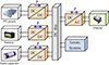 |
Figure 1 Electric power system for solar-powered vehicles. |
This study focuses on the PMSM motor and its corresponding DC/AC converter. The PMSM used in this research consists of three windings on the stator, along with permanent magnets either embedded inside the rotor for interior PMSM or mounted on the rotor surface for surface-mounted PMSM. In both cases, the continuous time model of the PMSM in the rotating coordinate system of dq-axis is represented by equations (1) and (2). The adoption of a rotating coordinate system, rather than the natural coordinate system, is a deliberate choice due to its ability to achieve decoupling control and effectively reduce the number of variables involved in the motor’s control scheme. This approach allows for enhanced control and improved efficiency of the PMSM, enabling precise manipulation of the motor’s performance and behavior. (1)
(1)
 (2)
(2)
To analyze the relationship between current and stator voltage, equations (1) and (2) can be expressed as shown in equations (3) and (4), respectively, with the dq-axis stator current selected as the state variable. (3)
(3)
 (4)
(4)
3 Conventional PMSM control
Within the realm of conventional PMSM control, numerous strategies exist in literature. However, in this particular study, our attention is directed towards the FOC and CDPC methods.
3.1 Field oriented control
Figure 2 illustrates the FOC for the dq-axis PMSM currents. This control strategy primarily focuses on precisely regulating the motor current components i d and i q . In this work, the d-axis reference value current is set to zero since the d-axis is aligned with the magnetic field of the permanent magnets. By setting the d-axis current to zero, the magnetic flux in the d-axis remains constant and aligned with the permanent magnet’s field, which ensures a maximum torque at the minimum current. The transverse stator current reference on the q-axis is computed via the external speed controller ensured by a PI controller. After that, PI controllers are used to regulate the d-axis and q-axis current components. The controller compares the desired current values with the actual currents and adjusts the voltage applied to the motor accordingly. Once the desired d–q current values are computed, they are transformed back to the stationary reference frame to generate the necessary voltage commands for the inverter that drives the motor. These voltage commands are used to modulate the inverter’s switching signals to control the motor.
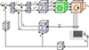 |
Figure 2 Block diagram for FOC. |
3.2 Conventional deadbeat predictive control
Figure 3 depicts the CDPC applied to the dq-axis currents of a PMSM. The primary objective of this control approach is to achieve precise regulation of the motor’s current components i d and i q . A PI controller is used to regulate the motor speed.
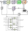 |
Figure 3 Block diagram for conventional deadbeat predictive control. |
The optimal voltage vector, which is applied to the PMSM through a Space Vector Modulation (SVM) process, is computed considering the PMSM state model (Eqs. (3) and (4)) and the Forward Euler discretization method (Eq. (5)). The obtained digital prediction equations are expressed by equations (6) and (7).![Mathematical equation: $$ \frac{\mathrm{d}{i}_{{dq}}(t)}{\mathrm{d}t}=\frac{{i}_{{dq}}[k+1]-{i}_{{dq}}[k]}{{T}_s}, $$](/articles/stet/full_html/2023/01/stet20230175/stet20230175-eq7.gif) (5)
(5)
![Mathematical equation: $$ {i}_d\left[k+1\right]=\left(1-\frac{R{T}_s}{L}\right){i}_d[k]+p{T}_s\omega [k]{i}_q[k]+\frac{{T}_s}{L}{U}_d[k], $$](/articles/stet/full_html/2023/01/stet20230175/stet20230175-eq8.gif) (6)
(6)
![Mathematical equation: $$ {i}_q\left[k+1\right]=\left(1-\frac{R{T}_s}{L}\right){i}_q[k]-p{T}_s\omega [k]{i}_d[k]+\frac{{T}_s}{L}{U}_q[k]-\frac{{p\phi }{T}_s}{L}\omega [k]. $$](/articles/stet/full_html/2023/01/stet20230175/stet20230175-eq9.gif) (7)
(7)
The CDPC is founded on the prediction criterion outlined in equations (8) and (9) for the d and q axes, respectively. This criterion ensures that the error between the motor current components (i
d
[k + 1] and i
q
[k + 1]) and their corresponding references (![Mathematical equation: $ {i}_d^{*}[k]$](/articles/stet/full_html/2023/01/stet20230175/stet20230175-eq10.gif) and
and ![Mathematical equation: $ {i}_q^{*}[k]$](/articles/stet/full_html/2023/01/stet20230175/stet20230175-eq11.gif) ) is minimized, ideally reduced to zero, as depicted in equations (8) and (9).
) is minimized, ideally reduced to zero, as depicted in equations (8) and (9).![Mathematical equation: $$ {i}_d[k+1]={i}_d^{\mathrm{*}}[k]\iff {i}_d[k+1]-{i}_d^{\mathrm{*}}[k]=0, $$](/articles/stet/full_html/2023/01/stet20230175/stet20230175-eq12.gif) (8)
(8)
![Mathematical equation: $$ {i}_q[k+1]={i}_q^{\mathrm{*}}[k]\iff {i}_q[k+1]-{i}_q^{\mathrm{*}}[k]=0. $$](/articles/stet/full_html/2023/01/stet20230175/stet20230175-eq13.gif) (9)
(9)
Considering the two previous equations, the reference voltages are expressed as follows:![Mathematical equation: $$ {U}_d^{\mathrm{opt}}[k]=a{i}_d^{\mathrm{*}}[k]+b{i}_d[k]-{pL\omega }[k]{i}_q[k], $$](/articles/stet/full_html/2023/01/stet20230175/stet20230175-eq14.gif) (10)
(10)
![Mathematical equation: $$ {U}_q^{\mathrm{opt}}[k]=a{i}_q^{\mathrm{*}}[k]+b{i}_q[k]+{pL\omega }[k]{i}_d[k]+{c\omega }[k], $$](/articles/stet/full_html/2023/01/stet20230175/stet20230175-eq15.gif) (11)
(11)
According to equations (10) and (11), the accuracy of current prediction relies heavily on the precise estimation and calibration of model parameters. When these parameters are correctly determined, the stator currents at the next sampling instant closely align with the predicted values, resulting in enhanced control performance. However, real-world conditions introduce various factors that can affect these parameters. Mechanical vibrations, magnetic saturation, temperature variations, and measurement errors are some of the key factors leading to changes in model parameters over time. These variations can significantly impact the control performance by introducing discrepancies between the predicted and actual currents. Consequently, the control system may not respond as expected, potentially leading to reduced efficiency and less accurate torque and speed control. In the following sections, we delve into the effects of parameter uncertainty on current prediction. The study will analyze and discuss how these uncertainties impact the overall control performance.
4 PMSM parameter uncertainty effects
Based on [10], the parameters that exert the most significant influence are resistance, inductance, and flux parameters. To explore the impact of parameter uncertainty on current prediction, we represent these parameters as follows: (12)
(12)
 (13)
(13)
 (14)
(14)
In case of parameter mismatch and based on equations (6) and (7), the current prediction model can be expressed as in equations (15) and (16).![Mathematical equation: $$ {i}_d^\mathrm{\prime}\left[k+1\right]=\left(1-\frac{{T}_s\left({R}_0+{\Delta }_R\right)}{{L}_0+{\Delta }_L}\right){i}_d[k]+p{T}_s\omega [k]{i}_q[k]+\frac{{T}_s}{{L}_0+{\Delta }_L}{U}_d[k], $$](/articles/stet/full_html/2023/01/stet20230175/stet20230175-eq20.gif) (15)
(15)
![Mathematical equation: $$ {i}_q^\mathrm{\prime}\left[k+1\right]=\left(1-\frac{{T}_s\left({R}_0+{\Delta }_R\right)}{{L}_0+{\Delta }_L}\right){i}_q[k]-p{T}_s\omega [k]{i}_d[k]+\frac{{T}_s}{{L}_0+{\Delta }_L}{U}_q[k]-\frac{p{T}_s\omega [k]\left({\phi }_0+{\Delta }_{\phi }\right)}{{L}_0+{\Delta }_L}. $$](/articles/stet/full_html/2023/01/stet20230175/stet20230175-eq21.gif) (16)
(16)
Finally, the prediction errors between the model subjected to parameter change given by equations (15) and (16) and the real model given by equations (8) and (9) is expressed as follows:![Mathematical equation: $$ {E}_d={i}_d^\mathrm{\prime}\left[k+1\right]-{i}_d\left[k+1\right]=\frac{{T}_s\left({R}_0{\Delta }_L+{L}_0{\Delta }_R\right)}{{L}_0\left({L}_0+{\Delta }_L\right)}{i}_d[k]-\frac{{T}_s{\Delta }_L}{{L}_0\left({L}_0+{\Delta }_L\right)}{U}_d[k], $$](/articles/stet/full_html/2023/01/stet20230175/stet20230175-eq22.gif) (17)
(17)
![Mathematical equation: $$ {E}_q={i}_q^\mathrm{\prime}\left[k+1\right]-{i}_q\left[k+1\right]=\frac{{T}_s\left({R}_0{\Delta }_L+{L}_0{\Delta }_R\right)}{{L}_0\left({L}_0+{\Delta }_L\right)}{i}_q[k]-\frac{{T}_s{\Delta }_L}{{L}_0\left({L}_0+{\Delta }_L\right)}{U}_q[k]+\frac{p{T}_s\omega [k]\left({\phi }_0{\Delta }_L-{L}_0{\Delta }_{\phi }\right)}{{L}_0\left({L}_0+{\Delta }_L\right)}. $$](/articles/stet/full_html/2023/01/stet20230175/stet20230175-eq23.gif) (18)
(18)
Figure 4 illustrates the correlation between the mismatch of the stator inductance and resistance and the d-axis current error E d . Figure 5 is presented the relationship between the mismatch of the stator inductance and resistance and the q-axis current error E q .
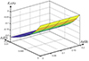 |
Figure 4 Relationship between the mismatch of resistance and inductance and the d-axis current error E d . |
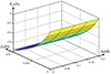 |
Figure 5 Relationship between the mismatch of resistance and inductance and the q-axis current error E q . |
Additionally, Figure 6 showcases the relationship between the flux-linkage mismatch and the q-axis current error E q . Upon analyzing these figures, it becomes evident that both current error E d and E q experience significant variations when any one motor parameter mismatches. The variation of a single parameter induces errors in the predicted currents, thus leading to a decrease in control performance.
 |
Figure 6 Relationship between the flux-linkage mismatch and the q-axis current error E q . |
5 Adaptive Deadbeat Predictive Control with consideration for stator resistance rise
For the used PMSM motor, the winding resistance of the stator is influenced by the internal temperature of the motor. During motor operation, various factors, such as current flowing through the windings and mechanical losses, contribute to the generation of heat. As the internal temperature of the motor increases, the resistance of the motor windings undergoes changes. The relationship between temperature and resistance in PMSM motors is typically described by the positive temperature coefficient of resistance. In simple terms, as the temperature rises, the resistance of the stator windings increases proportionally. This change in resistance due to temperature variations has significant implications for motor control and overall performance. With increasing temperature, the resistance also increases, which, in turn, affects the current flowing through the motor windings. Consequently, the torque and speed characteristics of the motor can be impacted. To address the influence of temperature on motor performance and ensure accurate control, real-time resistance adjustments are necessary. The adaptive control strategy takes into account the estimated value of the temperature (T) and dynamically adjusts the resistance according to the temperature changes, as described by equation (19) [18]. By incorporating temperature-compensated resistance adjustments into the motor control algorithm, the system can effectively adapt to varying operating conditions and temperature fluctuations, leading to enhanced motor performance and precise control. The real-time estimating of the temperature is treated in several references [19–21] and is not detailed in this paper. (19)
(19)
The proposed adaptive ADPC is illustrated in Figures 7 and 8. In this control scheme, additional input is introduced to the existing CDPC. This new input represents the real-time value of the actual stator resistance. To obtain this value, the PMSM winding temperature is measured using temperature sensors or can be estimated through sensor-less temperature estimation methods or a prediction approach [22–24]. Once the real-time stator resistance value is determined, it is subtracted from the predicted value based on equation (19). This deduction enables the control system to account for the influence of temperature on the motor winding resistance. By incorporating this adaptive approach, the ADPC can dynamically adjust the control parameters and compensate for changes in the stator resistance due to temperature variations. The integration of real-time temperature-based resistance adjustments enhances the ADPC’s ability to adapt to varying temperature conditions, ensuring more accurate and efficient motor control. This adaptive control strategy contributes to improved motor performance and robustness, enabling the PMSM to operate optimally across a wide range of operating temperatures.
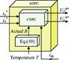 |
Figure 7 ADPC principle. |
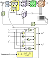 |
Figure 8 Block diagram for Adaptive Deadbeat Predictive Control. |
6 Simulation results and discussion
Simulations are established in MATLAB/Simulink. For simulation tests, several scenarios are used: the first one with a simple step reference input speed, and the second one with two driving cycle reference input speeds, namely, the Urban Dynamometer Driving Schedule (UDDS) driving cycle and the Economic Commission for Europe Regulation 15 (ECE R15) driving cycle. The studied vehicle is a golf car with 2–4 passengers. In fact, nowadays, this car is not limited to golf courses; it is used for short-distance trips in airports, businesses, universities, and residential areas. This vehicle, as well as its characteristics, are provided in Figure 9 and Table 1, respectively. The PMSM parameters are presented in Table 2.
PMSM and system parameters.
6.1 Simple step reference input speed
The simulation section is divided into two parts. The first part shows the effectiveness of the CDPC against the FOC. The second part proves the efficiency of the proposed ADPC compared to the CDPC in the case of stator resistance variation. During simulation, the rated speed of the PMSM is regulated to 50 rpm. Figures 10–12 present a comparison between PMSM comportment when applying FOC and CDPC. These figures illustrate the evolution of the currents i abc , i d and i q , respectively. As shown in both the three-phase current and the dq components current, CDPC results in fewer current harmonics.
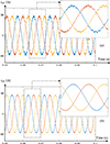 |
Figure 10 Simulation results of i abc currents in case of (a) FOC and (b) CDPC. |
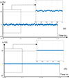 |
Figure 11 Simulation results of i d current component in case of (a) FOC and (b) CDPC. |
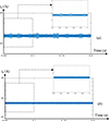 |
Figure 12 Simulation results of i q current component in case of (a) FOC and (b) CDPC. |
In order to show the robustness of the proposed control against stator resistance mismatch, an uncertainty equal to 5R is added to the real stator resistance. Figure 13 shows the evolution of the current i q in the case of the application of CDPC and ADPC for a speed rotation change at 0.1 s. As presented in this figure, the current ripple in the case of ADPC is reduced compared to the CDPC. Also, the current in the case of ADPC takes fewer time to attract its reference compared to the CDPC. Figure 14 presents the evolution of the current i d in the case of CDPC and ADPC for a speed rotation change at 0.1 s. As presented in this figure, the current i d is well equal to zero in the case of ADPC which is not the case for the CDPC.
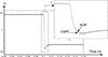 |
Figure 13 Simulation results of i q current with stator resistor mismatch in case of CDPC and ADPC. |
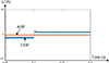 |
Figure 14 Simulation results of i d current with stator resistor mismatch in case of CDPC and ADPC. |
6.2 Driving cycle reference input speed
Real-world scenarios involve electric vehicles experiencing driving cycles of varying complexities, rather than simple-step inputs. These driving cycles, especially city driving cycles, are characterized by intricate patterns, random fluctuations, and sudden changes, which significantly amplify the challenges of effective control. In the subsequent section, the effectiveness of the proposed ADPC was evaluated using diverse international driving cycles. For the purpose of this study, the electric vehicle’s control system was subjected to two internationally recognized certified driving cycles: the UDDS driving cycle and the ECE R15 driving cycle. These selected driving cycles provide a comprehensive assessment of the vehicle’s behavior under different operational conditions, facilitating a rigorous evaluation of the control strategies.
6.2.1 UDDS driving cycle
Figure 15 shows the PMSM speed response for CDPC and ADPC and its reference when the UDDS driving cycle is applied in case of stator resistance mismatch. One can notice that there is almost a match between the ADPC speed and the reference compared to the CDPC speed. PMSM phase currents are shown in Figure 16. The zoom on that figure shows that they are pure sinusoidal and 120° apart. Figure 17 presents the PMSM i d and i q currents in the case of ADPC.
 |
Figure 15 PMSM speed response and its reference for UDDS driving cycle. |
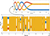 |
Figure 16 PMSM current response for UDDS driving cycle. |
 |
Figure 17 PMSM i d and i q current components for UDDS driving cycle. |
6.2.2 ECE R15 driving cycle
Figure 18 shows the speed response and its reference when the ECE R15 driving cycle is used as input speed reference and in the case of PMSM stator resistance uncertainty. As shown in this figure, the best results are obtained with the ADPC compared to the CDPC. Figures 19 and 20 present the PMSM current response and the PMSM i d and i q currents for the ECE R15 driving cycle in the case of ADPC.
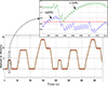 |
Figure 18 PMSM speed response and its reference for ECE R15 driving cycle. |
 |
Figure 19 PMSM current response for ECE R15 driving cycle. |
 |
Figure 20 PMSM i d and i q current components for ECE R15 driving cycle. |
In summary, the application of ADPC leads to results that closely align with the baseline compared to the utilization of conventional deadbeat predictive control.
7 Conclusion
This study introduces an Adaptive Deadbeat Predictive Control (ADPC) strategy for a Permanent Magnet Synchronous Motor (PMSM) integrated into a solar powered electric vehicle (SEV). The central aim of this control is to mitigate the impact of stator resistance mismatches. The core principle revolves around real-time control adaptation through the continuous estimation of the resistance value, considering the actual winding temperature. The simulation outcomes validate the effectiveness of the proposed ADPC strategy in enhancing control robustness against stator resistance variations. By offering dynamic adjustments to the control parameters based on the changing temperature and its effect on resistance, the ADPC demonstrates its potential to significantly improve the stability and performance of PMSMs in the context of SEVs. This approach holds promise for advancing the reliability and efficiency of electric vehicle propulsion systems, contributing to the broader objective of sustainable transportation. For further work, an experimental setup, given by Figure 21, will be used to illustrate the effectiveness of the proposed ADPC control strategy. It includes (1) an Integrated Permanent Magnet Synchronous Motor (PMSM) in the wheel functioning as the propulsion unit; (2) a microchip DC/AC power converter responsible for converting direct current from the power source into alternating current; (3) an incremental encoder system which provides instantaneous measurement of the wheel’s rotational speed; (4) a measurement board that provides current measurements and (5) Texas Instruments TI F28335 digital solution, which is used for the control algorithm implementation.
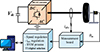 |
Figure 21 Experimental prototype. |
Acknowledgments
This work was supported by the Tunisian Ministry of High Education and Research under Grant LSE-ENIT-LR 11ES15 and funded in part by the Programme d’Encouragement des Jeunes Chercheurs (PEJC) (Code 21PEJC D6P10).
References
- Nezamuddin O.N., Nicholas C.L., Santos E.C.d. (2022) The problem of electric vehicle charging: state-of-the-art and an innovative solution, IEEE Trans. Intell. Transp. Syst. 23, 5, 4663–4673. https://doi.org/10.1109/TITS.2020.3048728. [CrossRef] [Google Scholar]
- El Harouri K., El Hani S., Naseri N., Elbouchikhi E., Benbouzid M., Skander-Mustapha S. (2023) Hybrid control and energy management of a residential system integrating vehicle-to-home technology, Designs 7, 2, 52. [CrossRef] [Google Scholar]
- Ben Said-Romdhane M., Skander-Mustapha S., Belhassen R. (2022) Adaptative deadbeat predictive control for PMSM based electric vehicle, in: 2022 IEEE International Conference on Electrical Sciences and Technologies in Maghreb (CISTEM), 26–28 October 2022, Tunis, Tunisia, pp. 1–6. https://doi.org/10.1109/CISTEM55808.2022.10043945. [Google Scholar]
- Ben Said-Romdhane M., Skander-Mustapha S. (2021) A review on vehicle-integrated photovoltaic panels, in: Motahhir S., Eltamaly A.M. (eds.), Advanced Technologies for Solar Photovoltaics Energy Systems. Green Energy and Technology, Springer, Cham. https://doi.org/10.1007/978-3-030-64565-6_12. [Google Scholar]
- Said-Romdhane M.B., Skander-Mustapha S., Slama-Belkhodja I. (2021) Analysis study of city obstacles shading impact on solar PV vehicle, in: 2021 4th International Symposium on Advanced Electrical and Communication Technologies (ISAECT), Dec. 6–8, 2021. https://doi.org/10.1109/ISAECT53699.2021.9668573. [Google Scholar]
- Ben Said-Romdhane M., Skander-Mustapha S., Slama-Belkhodja I., Robust control for energy storage system dedicated to solar-powered electric vehicle, in: Motahhir S. (eds.), Digital Technologies for Solar Photovoltaic Systems: From general to rural and remote installations. IET publisher, 2022. https://doi.org/10.1049/PBPO228E_ch13. [Google Scholar]
- Deng W., Zuo S. (2019) Electromagnetic vibration and noise of the permanent-magnet synchronous motors for electric vehicles: an overview, IEEE Trans. Transp. Electrification 5, 1, 59–70. https://doi.org/10.1109/TTE.2018.2875481. [CrossRef] [MathSciNet] [Google Scholar]
- Sain C., Banerjee A., Biswas P.K., Padmanaban S. (2020) A state-of-the-art review on solar-powered energy-efficient PMSM drive smart electric vehicle for sustainable development, in: A. Bhoi, K. Sherpa, A. Kalam, G.S. Chae (eds.), Advances in Greener Energy Technologies. Green Energy and Technology, Springer, Singapore. https://doi.org/10.1007/978-981-15-4246-6_15. [Google Scholar]
- Sreejith R., Singh B. (2019) Intelligent nonlinear sensorless predictive field oriented control of PMSM drive for three wheeler hybrid solar PV-battery electric vehicle, IEEE Transportation Electrification Conference and Expo (ITEC), pp. 1–6. https://doi.org/10.1109/ITEC.2019.8790458. [Google Scholar]
- Ton T.-D., Hsieh M.-F., Chen P.-H. (2021) A novel robust sensorless technique for field-oriented control drive of permanent magnet synchronous motor, IEEE Access 9, 100882–100894. https://doi.org/10.1109/ACCESS.2021.3097120. [CrossRef] [Google Scholar]
- Ding H., Zou X., Li J. (2022) Sensorless control strategy of permanent magnet synchronous motor based on fuzzy sliding mode observer, IEEE Access 10, 36743–36752. https://doi.org/10.1109/ACCESS.2022.3164519. [CrossRef] [Google Scholar]
- Wang W., Shen H., Hou L., Gu H. (2019) H∞ robust control of permanent magnet synchronous motor based on PCHD, IEEE Access 7, 49150–49156. https://doi.org/10.1109/ACCESS.2019.2893243. [CrossRef] [Google Scholar]
- Zhang C., Wu G., Rong F., Feng J., Jia L., He J., Huang S. (2018) Robust fault-tolerant predictive current control for permanent magnet synchronous motors considering demagnetization fault, IEEE Trans. Ind. Electron. 65, 7, 5324–5334. https://doi.org/10.1109/TIE.2017.2774758. [CrossRef] [MathSciNet] [Google Scholar]
- Rabbi S.F., Halloran M.P., LeDrew T., Matchem A., Rahman M.A. (2016) Modeling and V/F control of a hysteresis interior permanent-magnet motor, IEEE Trans. Ind. Appl. 52, 2, 1891–1901. https://doi.org/10.1109/TIA.2015.2505666. [Google Scholar]
- Li Y., Li Y., Wang Q. (2020) Robust predictive current control with parallel compensation terms against multi-parameter mismatches for PMSMs, IEEE Trans. Energy Convers. 35, 4, 2222–2230. https://doi.org/10.1109/TEC.2020.3002274. [CrossRef] [Google Scholar]
- Zhang X., Zhang L., Zhang Y. (2019) Model predictive current control for PMSM drives with parameter robustness improvement, IEEE Trans. Power Electron. 34, 2, 1645–1657. https://doi.org/10.1109/TPEL.2018.2835835. [CrossRef] [Google Scholar]
- Long J., Yang M., Chen Y., Liu K., Xu D. (2021) Current-controller-free self-commissioning scheme for deadbeat predictive control in parametric uncertain SPMSM, IEEE Access 9, 289–302. https://doi.org/10.1109/ACCESS.2020.3043751. [CrossRef] [Google Scholar]
- Boglietti A., Carpaneto E., Cossale M., Vaschetto S. (2016) Stator-winding thermal models for short-time thermal transients: definition and validation, IEEE Trans. Ind. Electron. 63, 5, 2713–2721. https://doi.org/10.1109/TIE.2015.2511170. [CrossRef] [Google Scholar]
- Kral C., Haumer A., Lee S.B. (2014) A practical thermal model for the estimation of permanent magnet and stator winding temperatures, IEEE Trans. Power Electron. 29, 1, 455–464. https://doi.org/10.1109/TPEL.2013.2253128. [CrossRef] [Google Scholar]
- Dariusz C., Jakub G., Krzysztof K. (2021) Machine learning for sensorless temperature estimation of a BLDC motor, Sensors 21, 14, 4655. https://doi.org/10.3390/s21144655. [CrossRef] [PubMed] [Google Scholar]
- Li Z., Feng G., Lai C., Li W., Kar N.C. (2021) Current injection-based simultaneous stator winding and PM temperature estimation for dual three-phase PMSMs, IEEE Trans. Ind. Appl. 57, 5, 4933–4945. https://doi.org/10.1109/TIA.2021.3091664. [CrossRef] [Google Scholar]
- Ding H., Gong X., Gong Y. (2020) Estimation of rotor temperature of permanent magnet synchronous motor based on model reference fuzzy adaptive control, Math. Prob. Eng. 1–11. [Google Scholar]
- Guo H., Ding Q., Song Y., Tang H., Wang L., Zhao J. (2020) Predicting temperature of permanent magnet synchronous motor based on deep neural network, Energies 13, 18, 4782–4796. [CrossRef] [Google Scholar]
- Jun B.S., Park J.S., Choi J.H., Lee K.D., Won C.Y. (2018) Temperature estimation of stator winding in permanent magnet synchronous motors using d-axis current injection, Energies 11, 8, 2033–2047. [CrossRef] [Google Scholar]
- https://wulingauto.en.made-in-china.com/product/asEnyWhDqQRL/China-48V3kw-AC-Asynchronous-Motor-Electric-Golf-Cart-2-4-Seats.html. [Google Scholar]
All Tables
All Figures
|
Figure 1 Electric power system for solar-powered vehicles. |
| In the text | |
|
Figure 2 Block diagram for FOC. |
| In the text | |
|
Figure 3 Block diagram for conventional deadbeat predictive control. |
| In the text | |
|
Figure 4 Relationship between the mismatch of resistance and inductance and the d-axis current error E d . |
| In the text | |
|
Figure 5 Relationship between the mismatch of resistance and inductance and the q-axis current error E q . |
| In the text | |
|
Figure 6 Relationship between the flux-linkage mismatch and the q-axis current error E q . |
| In the text | |
|
Figure 7 ADPC principle. |
| In the text | |
|
Figure 8 Block diagram for Adaptive Deadbeat Predictive Control. |
| In the text | |
 |
Figure 9 Electric golf car 2–4 seats [25]. |
| In the text | |
|
Figure 10 Simulation results of i abc currents in case of (a) FOC and (b) CDPC. |
| In the text | |
|
Figure 11 Simulation results of i d current component in case of (a) FOC and (b) CDPC. |
| In the text | |
|
Figure 12 Simulation results of i q current component in case of (a) FOC and (b) CDPC. |
| In the text | |
|
Figure 13 Simulation results of i q current with stator resistor mismatch in case of CDPC and ADPC. |
| In the text | |
|
Figure 14 Simulation results of i d current with stator resistor mismatch in case of CDPC and ADPC. |
| In the text | |
|
Figure 15 PMSM speed response and its reference for UDDS driving cycle. |
| In the text | |
|
Figure 16 PMSM current response for UDDS driving cycle. |
| In the text | |
|
Figure 17 PMSM i d and i q current components for UDDS driving cycle. |
| In the text | |
|
Figure 18 PMSM speed response and its reference for ECE R15 driving cycle. |
| In the text | |
|
Figure 19 PMSM current response for ECE R15 driving cycle. |
| In the text | |
|
Figure 20 PMSM i d and i q current components for ECE R15 driving cycle. |
| In the text | |
|
Figure 21 Experimental prototype. |
| In the text | |
Current usage metrics show cumulative count of Article Views (full-text article views including HTML views, PDF and ePub downloads, according to the available data) and Abstracts Views on Vision4Press platform.
Data correspond to usage on the plateform after 2015. The current usage metrics is available 48-96 hours after online publication and is updated daily on week days.
Initial download of the metrics may take a while.