")
")
| Issue |
Sci. Tech. Energ. Transition
Volume 78, 2023
|
|
|---|---|---|
| Article Number | 31 | |
| Number of page(s) | 15 | |
| DOI | https://doi.org/10.2516/stet/2023026 | |
| Published online | 31 October 2023 | |
Review Article
Metamodeling the optimal total revenues of the short-term optimization of a hydropower cascade under uncertainty
1
Compagnie Nationale du Rhône, Lyon 69004, France
2
Université de Lyon, UMR 5208, École Centrale de Lyon, Institut Camille Jordan, Lyon 69134, France
* Corresponding author: This email address is being protected from spambots. You need JavaScript enabled to view it.
Received:
28
June
2022
Accepted:
30
August
2023
Abstract
This paper deals with the optimization of the short-term production planning of a real cascade of run-of-river hydropower plants. Water inflows and electricity prices are subject to data uncertainty and they are modeled by a finite set of joint scenarios. The optimization problem is written with a two-stage stochastic dynamic mixed-integer linear programming formulation. This problem is solved by replacing the value function of the second stage with a surrogate model. We propose to evaluate the feasibility of fitting the surrogate model by supervised learning during a pre-processing step. The learning data set is constructed by Latin hypercube sampling after discretizing the functional inputs. The surrogate model is chosen among linear models and the dimension of the functional inputs is reduced by principal components analysis. Validation results for one simplified case study are encouraging. The methodology could however be improved to reduce the prediction errors and to be compatible with the time limit of the operational process.
Key words: Uncertainty quantification / Optimization / Hydropower plant management / Surrogate modeling
© The Author(s), published by EDP Sciences, 2023
 This is an Open Access article distributed under the terms of the Creative Commons Attribution License (https://creativecommons.org/licenses/by/4.0), which permits unrestricted use, distribution, and reproduction in any medium, provided the original work is properly cited.
1 Introduction
Managing a cascade of hydropower plants involves planning in advance its total power generation, especially for bidding the production on power markets. Short-term production planning of the cascade refers to the detailed operational scheduling of the hydropower plants within a time horizon of a few days and with a high time resolution [1]. A short-term production plan of the cascade is established to allocate the production between the hydropower plants and over the time horizon. This problem is part of the operational process of the cascade.
The total power generation of the cascade is sold on power markets. Short-term production planning is in relation to day-ahead market in which contracts are hourly power generation for physical delivery the following day. Market participants submit their bids for each hour of the following day, before the market closing. The hourly day-ahead prices for the following day are settled just after the closing time by the market clearing to meet the balance between sale and purchase offers, reflecting the need for balance between supply and demand on the power grid during the following day. The hourly day-ahead commitments are then defined according to the day-ahead bids and prices, and they are added to the long-term commitments (e.g., bilateral contracts). Real-time operation of the cascade is performed to ensure physical delivery of the commitments to the extent possible. Deviations between real delivery and commitments are called imbalances, and they are financially penalized.
If the power modulation capacity of the cascade is significant (large reservoirs), then hydrological flows have little impact on short-term hydropower production. In this case, the operational process could consist of first deciding the day-ahead bids and then establishing the short-term production plan according to that decision while limiting imbalances. Otherwise, if the power modulation capacity of the cascade is insignificant (perfect run-of-river hydropower plants), then the short-term hydropower production is strongly influenced by hydrological flows. In this case, the operational process could consist of first deciding the short-term production plan and then deducing the day-ahead bids by computing the hourly total energy of the production plan. In this paper, we consider an intermediate case of a run-of-river hydropower cascade for which the decision of the day-ahead bids and the decision of the short-term production can both be obtained simultaneously. This is done by solving the optimization problem that maximizes the total revenues obtained by selling the day-ahead bids and by penalizing imbalances, while complying with the physical models (hydraulic modeling and hydropower generation) and with operational requirements.
Water inflows and day-ahead prices are parameters of the optimization problem. They are both subject to data uncertainty because they inherit uncertainties of weather situations and market conditions over the time horizon. The deterministic framework, based on a single estimation of the uncertain parameters, may lead to a solution that is sub-optimal or even not feasible with the real-time observed parameters. Of course, the operational process can deal with this issue by updating the production plan at several regular times every day as uncertain information evolves over time. In the deterministic framework, however, this updating process of the production plan according to data uncertainty cannot be anticipated. That is rather the purpose of the stochastic framework, based on a mathematical representation of the uncertain parameters, for which several approaches are presented in the literature for similar optimization problems in the field of energy, e.g., in the reviews [2–4]. In this paper, we consider a two-stage stochastic dynamic programming formulation for which data uncertainty is modeled by a set of scenarios. The first stage relates to the decision of the day-ahead bids and the reference production plan. The second stage relates to the adaptation of the reference production plan with respect to the scenario, i.e., future possible updates and re-optimizations of the production plan so that it is always applicable and optimal as uncertainty information evolves over time. The two stages have a Mixed-Integer Linear Programming (MILP) formulation.
Solving this stochastic optimization problem within a time-constrained operational process is, however, quite challenging because of the size and complexity of the problem due to the detailed operational constraints and to the number of scenarios. Several approaches are presented in the literature to tackle this issue. They are often based on a decomposition scheme on the stages (e.g., L-shaped algorithm, Stochastic Dual Dynamic Programming) where the optimal value function of the second stage is approximated within an incremental procedure during the solving step of the optimization problem [5–8]. They have the advantage of being adaptive because they tend to reduce approximation errors of the value function around the optimality region. Other decomposition schemes proposed in the literature are based on the scenarios (e.g., Progressive Hedging [9]) or on space (e.g., Lagrangian decomposition [10, 11]). All these decomposition approaches are iterative algorithms. They are widely used for solving two-stage stochastic programming problems in the linear framework, especially in the field of unit commitment under uncertainty [4]. Some of them can be adapted to the integer framework, but with more restrictions on the problem formulation, such as a binary first stage or a pure integer second stage [12–16]. Therefore stochastic integer programming problems are generally relaxed before using a linear decomposition algorithm. For our problem, a linear relaxation would require a strong approximation of the underlying physical model, which could be unsuitable for real application in the operational process.
In this paper, we aim to evaluate the feasibility of using supervised learning during a pre-processing step instead of using an existing decomposition approach. Most of the complexity of the problem is deported to the pre-processing step. This has two main advantages:
-
the pre-processing step can be performed offline in advance and can fully exploit parallel computing,
-
the underlying physical model is not approximated.
The pre-processing step consists of constructing a learning data set and fitting a surrogate model (also called metamodel) of the optimal value function of the second stage. After the pre-processing step, the stochastic optimization problem is solved by replacing the optimal value function of the second stage with the surrogate model. The proposed methodology is relevant if prediction errors of the surrogate model are less than the requested MIP gap for the optimal solution, and if computation time is compatible with a use in real operations.
The inputs of the surrogate model are composed of the non-anticipative decision variables of the first stage and the scenario. This raises two main issues for constructing the design of experiments and fitting the surrogate model. The first issue is due to the functional structure of the two inputs, which can be tackled by dimension reduction [17–20]. The second issue is due to the non-explicit formulation of the domain of the input related to the non-anticipative decision variables, since it is only defined by MILP constraints. In the literature, the domain of the inputs is generally perfectly known or at least given by a sample of observations.
The outline of this paper is the following. Section 2 introduces the case study used throughout the paper, and it describes the mathematical formulation of the optimization problem and the role of the surrogate model. Sections 3 and 4 present the methodological approach for fitting the surrogate model by using the case study for illustrative purposes, considering respectively the design of experiments and the metamodeling process. Section 5 raises some discussions about the proposed methodology for solving the stochastic optimization problem.
2 Methodological approach
2.1 Motivating case
The methodology described in this paper is strongly related to real operations carried out by CNR (Compagnie Nationale du Rhône1), a French renewable electricity producer that operates in particular a cascade of 18 hydropower plants along the Rhône river (see Fig. 1), representing around 3000 MW of installed capacity (in 2021).
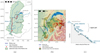 |
Figure 1 CNR’s hydropower plants along the Rhône river. (a) Rhône river, (b) upper part of the Rhône river and (c) scheme of the Rhône cascade. |
Apart from the first upstream hydropower plant, the other hydropower facilities are run-of-river, i.e., they can store a very limited amount of water compared to their average daily flow. The run-of-river hydropower plants allow only a very limited modulation of their outflows in comparison with their inflows for producing a bit more or less energy during a few hours. The power modulation capacity of each hydropower plant is small but sufficient to consider short-term economical optimization of the overall cascade in the day-ahead market. Since the hydropower plants influence each other through hydraulic propagation and water balance equations, the challenge for economic optimization is to synchronize discharges at each hydropower plant so that the total power generation of the cascade is in line with electricity prices to maximize total revenues [21]. Economical optimization is performed in advance through short-term production planning of the cascade, which is repeated every day at several regular times with an updated situation (input data, initial conditions of the Rhône river, and user parameters). A numerical optimizer for decision support can be used for this purpose.
In this paper, we consider the case study defined by the historical situation on 2014–04–26 at 11:00 a.m. (local time) for illustrative purposes. The case study is simplified by considering only the upper part of the Rhône river, i.e., the first I = 6 upstream hydropower plants (see Fig. 1b). Production plans of the 12 other hydropower plants of the cascade are supposed to be fixed but their power generation is counted in the total power generation. Let  denote the set of indices of every hydropower plant along the cascade.
The time horizon is supposed to be discretized into T = 360 regular time buckets of duration δt = 10 min. Let  denote the set of indices of every time bucket. We assume that the production plan cannot be changed for the next hour after the present time because of the time delay required for establishing the production plan and making changes in operations. Thus the time horizon begins on 2014–04–26 at 12:00 a.m. and it ends at the end of 2014–04–28 (+60 h). For simplification, we consider that water inflows and day-ahead prices forecasts start on 2014–04–26 at 12:00 a.m. like the time horizon, and that values between the present time (2014–04–26 11:00) and the beginning of the time horizon (2014–04–26 12:00) are observations. In the operational process, the forecasts would have started at the present time. Note that, due to the time delay of water propagation, a past time horizon is necessary in practice to define the initial conditions of the cascade.
Data uncertainty on water inflows at each hydropower plant over the time horizon is estimated by a uniformly distributed sample of 50 elements in ℝIT derived from an ensemble forecast of the hourly measured inflows of the 6 main natural tributaries taking part in the upper Rhône river that ensures reliability and correlations in space and time [22] (see Fig. 2a). Data uncertainty on unmeasured inflows is not considered in this paper. Likewise, data uncertainty on day-ahead prices is estimated by a uniformly distributed sample of 50 elements in ℝT from a simple quantile error model that ensures reliability and temporal autocorrelations (see Fig. 2b). Note that day-ahead prices are constant on every hour of the time horizon since they have hourly values. The two samples are then independently combined to build a uniformly distributed sample of N = 50 × 50 = 2500 joint scenarios. Therefore data uncertainty is modeled by a finite random variable  on some probability space (Ω, ℱ, ℙ) with values in ℝIT × ℝT. We denote by ξ
n
= (a
n
, π
n
) ∈ ℝIT × ℝT, for n ∈ {1,...,N}, the joint scenarios (elements of
on some probability space (Ω, ℱ, ℙ) with values in ℝIT × ℝT. We denote by ξ
n
= (a
n
, π
n
) ∈ ℝIT × ℝT, for n ∈ {1,...,N}, the joint scenarios (elements of  ) with their corresponding probabilities
 ![Mathematical equation: $ {p}_n=\mathbb{P}\left[\widehat{\mathrm{\Xi }}={\xi }_n\right]=1/N$](/articles/stet/full_html/2023/01/stet20220096/stet20220096-eq5.gif) . Throughout the paper,
. Throughout the paper,  stands for the expectation with respect to the probability space (Ω, ℱ, ℙ).
 |
Figure 2 Example of the ensemble forecasts (grey lines) taking part in the case study, the deterministic forecasts (thick blue lines), and the observations that were known at the present time (red lines). The ensemble forecasts for water inflows and day-ahead prices have 50 members each. The vertical dashed lines represent the beginning of the time horizon on 2014-04-26 12:00 (local time). For reasons of confidentiality, the forecast values of day-ahead prices are arbitrarily scaled. (a) Water inflows from the six natural tributaries taking part in the upper Rhône river over the time horizon and (b) day-ahead electricity prices over the time horizon. |
2.2 Short-term production planning
2.2.1 Feasible solutions
A solution to short-term production planning is a decision of a couple of
-
the next day-ahead bids, i.e., the hourly production to be sold in the day-ahead market and that would be added to the commitments,
-
the hydropower production plan, i.e., the allocation of every variable that takes part in physical models and operational requirements (imbalances, discharges, stream flows, powers, storage volumes, etc.) at each hydropower facility (see Fig. 1c) and over the time horizon.
The next-day-ahead bids and the production plan are mutually dependent on imbalances, i.e., deviations between production and commitments, that are allowed but financially penalized.
All variable values that define a solution are combined into a large vector x ∈ ℝr, where  is the problem size (i.e., the number of decision variables), r is
  . For the case study, r ≈ 500,000.
A solution is said to be feasible if its hydropower production plan complies with physical models, operational requirements, and next-day-ahead bids. These conditions are written as constraints on the solution. Some parameters depend on the scenario because water inflows appear in water balance equations that ensure the physical continuity of the cascade in time and space. For an example of typical constraints for hydropower production planning, see Appendix A or more generally the references in [4].
In this paper, constraints are supposed to be mixed-integer linear. In particular, hydropower generation is supposed to be piecewise linear with water discharges, and the net water heads are supposed to be independent of volumes. It should be noted that those strong assumptions may lead to non-negligible evaluation errors on power generation, but these deviations are acceptable in practice for the case study. Moreover, water time delays, bounds on volumes, and minimal final volumes are considered as parameters, i.e., they do not vary with the solution. Let  denote the (closed) set of all feasible solutions with respect to a generic scenario ξ = (a, π) ∈ ℝIT × ℝT. In the sequel, the set
  is assumed to be bounded for every ξ ∈ ℝIT × ℝT, and also nonempty if
  .
.
2.2.2 Total revenues
Let  be a feasible solution for a generic scenario ξ = (a, π) ∈ ℝIT × ℝT. Subtracting a constant from the total revenues if necessary, we may assume that the entire total power generation of the cascade is sold in the day-ahead market and long-term commitments are set to zero (see Fig. 3). Defining the total revenues then involves two types of interdependent decision variables: next-day-ahead bids and imbalances. Their planned values are given by some components of the solution x. Let b
t
(x) ∈ ℝ, for
be a feasible solution for a generic scenario ξ = (a, π) ∈ ℝIT × ℝT. Subtracting a constant from the total revenues if necessary, we may assume that the entire total power generation of the cascade is sold in the day-ahead market and long-term commitments are set to zero (see Fig. 3). Defining the total revenues then involves two types of interdependent decision variables: next-day-ahead bids and imbalances. Their planned values are given by some components of the solution x. Let b
t
(x) ∈ ℝ, for  , denote the values of the components related to the next day-ahead bids of the solution x over the time horizon. Let
  and
and  , for
, for  , denote the values of the components related to respectively positive and negative imbalances over the time horizon. These decision variables are linked together by the constraints in Appendix A.3.
 |
Figure 3 Example of the planned total power generation of a solution |

The total revenues f(x, ξ) ∈ ℝ of the solution x ∈ ℝr for the scenario ξ = (a, π) ∈ ℝIT × ℝT is then defined by (1)where
  and
and  are respectively positive and negative imbalance prices, supposed to be evaluated by downgrading day-ahead prices π ∈ ℝT that come from the scenario ξ, i.e., π
+ = (1 − κ
+)π and π
− = (1 + κ
−)π, with (κ
+, κ
−) ∈ (0, 1)2. For the case study, κ
+ = κ
− = 0.05. It should be noted that the total revenues defined in equation (1) is linear with the solution, since b
t
,
are respectively positive and negative imbalance prices, supposed to be evaluated by downgrading day-ahead prices π ∈ ℝT that come from the scenario ξ, i.e., π
+ = (1 − κ
+)π and π
− = (1 + κ
−)π, with (κ
+, κ
−) ∈ (0, 1)2. For the case study, κ
+ = κ
− = 0.05. It should be noted that the total revenues defined in equation (1) is linear with the solution, since b
t
,  and
and  , for
, for  , are linear projections onto some components of ℝr. For instance, for every
  , there exists some j0 ∈ {1,...,r} such that
The same applies with  and
and  , for
, for  .
.
2.2.3 Optimization problem
The deterministic short-term production planning problem consists of finding a feasible solution that maximizes the total revenues, with respect to a single reference scenario ξ0 = (a0, π0) ∈ ℝIT × ℝT. In practice, the reference scenario is obtained from operational deterministic forecasts which are completed with expertise (see blue curves in Fig. 2). The mathematical formulation is then the following MILP problem (2)where
  is supposed to be nonempty. For the case study, the MILP problem (2) is implemented in GAMS and solved with the CPLEX MIP solver. This optimizer is used within CNR’s operational process as a numerical decision support tool.
Even in the stochastic framework, we want the optimizer to give a unique feasible solution with respect to the reference scenario ξ0 = (a0, π0) ∈ ℝIT × ℝT used in the deterministic framework (Eq. (2)). The reason for this choice is that the reference scenario is composed of operational deterministic forecasts that are completed with expertise while providing expertise for probabilistic forecasts is an ongoing research [23]. In consequence, data uncertainty is not considered in the constraints that define the set of feasible solutions, but only in the total revenues to account for the impact of adapting the production plan with respect to the effective scenario. More precisely, the stochastic formulation considered in this paper is the following two-stage stochastic dynamic programming problem![Mathematical equation: $$ \underset{{\mathbf{x}}_0\in \mathcal{X}({\xi }_0)}{\mathrm{max}}\left\{{\alpha }_0f\left({\mathbf{x}}_0,{\xi }_0\right)+\left(1-{\alpha }_0\right)\mathbb{E}[Q\left(b{(\mathbf{x}}_0\right),\widehat{\mathrm{\Xi }})]\right\}, $$](/articles/stet/full_html/2023/01/stet20220096/stet20220096-eq30.gif) (3)
(3)
where:
-
b: ℝr → ℝ24 is the function that gives the upcoming hourly day-ahead bids of a solution, i.e., the linear mapping defined by
 where (h1,…,h24) ∈
  are the first-time buckets of every hour of delivery of the upcoming day-ahead bids. For the case study, h
j
= 73 + 6(j − 1), for j ∈ {1,…,24}.
are the first-time buckets of every hour of delivery of the upcoming day-ahead bids. For the case study, h
j
= 73 + 6(j − 1), for j ∈ {1,…,24}.
-
Q: ℝ24 × (ℝIT × ℝT) → [−∞,+∞) is the optimal value function of the second stage defined by
 (4)The optimal value function Q represents the optimal total revenues that can be achieved from a given decision of the upcoming day-ahead bids under the assumption that a given scenario effectively occurs. It should be noted that the optimal value function Q depends on the situation and user parameters, just like the scenario and the set of feasible solutions.
-
α0 ∈ [0, 1] is a weight for the reference scenario ξ0, that can be computed, for example, as the weight of a central cluster of the scenarios in
 . If α0 = 1, then the stochastic and deterministic formulations merge. If α0 = 0, then the reference scenario is not used in the objective function, leading to a more classical stochastic formulation. If α0 ∈ (0, 1), then the objective function is a compromise between the total revenues when no update of the production plan is required (i.e., when the reference scenario perfectly occurs) and the optimal total revenues after adapting the production plan for the scenarios. For the case study, the weight of the reference scenario ξ0 is arbitrarily set to α0 = 0.5.
The stochastic problem in equation (3) can be written with the following equivalent large MILP problem (5)which is too large to be tractable for the case study with the CPLEX MIP solver.
The stochastic formulation is similar to that of two-stage stochastic programming (with recourse) because it is based on a scenario tree with 2 stages. The first stage involves the reference scenario to define the production plan and the bids in the upcoming day-ahead market. The second stage involves all the probabilistic scenarios, without transition, to anticipate the future possible updates and re-optimizations of the production plan in view of the decision of the day-ahead bids made at the first stage. The non-anticipativity constraints appear in the bids in the upcoming day-ahead market that have to be compatible with the reference scenario. The dependence of the second stage on the first stage is also the basis of stochastic dynamic programming. The optimization problems of the 2 stages only differ by the choice of the scenario and by fixing the bids in the upcoming day-ahead market in the second stage.
2.3 Proposed methodology
The main issue in solving the stochastic programming problem in equation (3) is that the function Q needs to be evaluated a lot of times with different upcoming day-ahead bids in  and different scenarios in
  , while an evaluation of the function Q requires significant computation time for solving a large MILP problem (see Eq. (4)). This paper focuses on fitting a real-valued surrogate model
  on ℝ24 × (ℝIT × ℝT) that is fast to evaluate, and that is an approximation of Q on
  ,
, (6)
(6)
The condition in equation (6) ensures in particular that![Mathematical equation: $$ \mathbb{E}\left[\widehat{Q}\left({b}_0,\widehat{\mathrm{\Xi }}\right)\right]\approx \mathbb{E}\left[Q\left({b}_0,\widehat{\mathrm{\Xi }}\right)\right],\hspace{0.5em}\forall {b}_0\in {\mathcal{B}}_0, $$](/articles/stet/full_html/2023/01/stet20220096/stet20220096-eq41.gif) thus the problem
thus the problem![Mathematical equation: $$ \underset{{\mathbf{x}}_{\mathbf{0}}\in \mathcal{X}({\xi }_0)}{\mathrm{max}}\left\{{\alpha }_0f({\mathbf{x}}_0,\enspace {\xi }_0)\enspace +\enspace (1-{\alpha }_0)\mathbb{E}[\widehat{Q}(b({\mathbf{x}}_0),\enspace \widehat{\mathrm{\Xi }})]\right\} $$](/articles/stet/full_html/2023/01/stet20220096/stet20220096-eq42.gif) (7)is an approximation of the stochastic problem in equation (3).
(7)is an approximation of the stochastic problem in equation (3).
For a fixed scenario  is the value function of the MILP problem in equation (4), so it is piecewise linear with a finite number of discontinuity breakpoints [24, 25]. More details about the structure of this kind of function are presented in [26]. If the surrogate function
  is chosen among piecewise linear functions, then the problem in equation (7) has a MILP formulation with a much smaller dimension than the large MILP problem in equation (5).
In this paper, we propose to fit the surrogate model  every new situation during a pre-processing step by supervised learning based on a limited collection of evaluations of the function Q. The issue is that the computation time of the pre-processing step and solving the problem in equation (7) has to be compatible with the operational process. The pre-processing step is divided into two main successive substeps: constructing the learning data set (Sect. 3) and fitting the surrogate model (Sect. 4).
The learning data set is composed of couples of  at which the optimal value function Q is evaluated. The issue is that the set
  of acceptable upcoming day-ahead bids is not known with an explicit formulation but with the MILP constraints of the set
  . It is then difficult to characterize the elements of
  or to draw some of them. Thus we aim at approximating the set
  by a simpler set
  . A design of experiments is then constructed to select some couples of the input data set
  at which the optimal value function Q is evaluated. The difficulty is that the inputs have a functional structure, and the set of selected points needs to properly describe the input data set while being small enough to restrain computation time.
The type of the surrogate model is chosen according to its implementation in equation (7), the structure of the exact function Q, and the computation time of fitting. The issue is that the inputs have a large dimension, making it difficult to fit a model on a small learning data set. A dimension reduction of the inputs is then performed and the surrogate model is fitted on the reduced inputs.
3 Computational design
3.1 Discretization of day-ahead bids
We propose to approximate the set  by a finite set
  , where (b1,…,b
M
) ∈ (ℝ24)M (M ∈ ℕ) is a sample obtained by selecting the effective day-ahead bids associated to M past historical situations that are close to the situation at hand among a set of consecutive previous historical situations. This sampling process is inspired by analogue-based weather forecasting [27, 28] and it mainly consists of comparing situations one with another.
, where (b1,…,b
M
) ∈ (ℝ24)M (M ∈ ℕ) is a sample obtained by selecting the effective day-ahead bids associated to M past historical situations that are close to the situation at hand among a set of consecutive previous historical situations. This sampling process is inspired by analogue-based weather forecasting [27, 28] and it mainly consists of comparing situations one with another.
Since a lot of parameters change from one situation to another, it is crucial to carefully assess what parameters are to be considered for the distance used to compare similarities among situations. Moreover, the sampling size M is arbitrary and it has to be carefully chosen. In the sequel, the methodology to make these choices is described for the hydropower cascade of the case study defined in Section 2.1, but it can be adapted to another hydropower cascade.
In order to measure similarities among situations, we choose to separately test the three following parameters:
-
the hourly observation of total active power during the previous day,
-
the hourly deterministic forecast of cumulative measured water inflows of all tributaries along the Rhône river for the following day,
-
the hourly deterministic forecast of day-ahead prices for the following day.
The M closest situations to the situation at hand with respect to the chosen comparison distance are selected among the set of the 1000 consecutive previous historical situations. The sample (b1,…,b M) ∈ (ℝ24)M is then obtained by getting the effective day-ahead bids associated with the M-selected situations.
In this paper, the quality of discretization of the set  refers to the statistical consistency of the sample (b1,…,b
M
) with the effective day-ahead bids
refers to the statistical consistency of the sample (b1,…,b
M
) with the effective day-ahead bids  of the situation at hand. For verification, we compute the Continuous Ranked Probability Score (CRPS), a classical score used in probabilistic weather forecasting [29–31]. The CRPS compares the empirical cumulative density function of the sample with that of the observation, i.e., the effective day-ahead bids here. More precisely, the CRPS is the positive score defined by
 where H: ℝ → {0, 1} is the Heaviside function defined by H(u) = 1 if u ≥ 0 and H(u) = 0 otherwise, for u ∈ ℝ. The closer the CRPS is to zero, the better the quality of discretization is.
To limit the computation time required when considering a new situation, we aim to find the comparison parameter and the sampling size that provide the best overall quality of discretization for every situation (and not only for the particular situation at hand). For this purpose, the sampling process of day-ahead bids is repeated on a testing data set of daily situations in 2019 (365 days), considering successively the three comparison parameters and different values of the sampling size M. The testing criterion is the mean of CRPS on the testing data set that we aim to minimize. The results are presented in Figure 4. It turns out that the best quality is attained with the distance based on the L 1-norm of the cumulative water inflows (second comparison parameter) and with M = 21. For convenience, however, the sampling size is set to M = 20, without having a significant impact on the mean of CRPS.
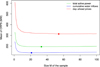 |
Figure 4 The average CRPS as a function of the size M of the sample for the three comparison parameters. A minimum is attained at M = 21 with the distance based on the L 1-norm of the cumulative water inflows (second comparison parameter). |
It should be noted that the finite set  obtained by the sampling process is not necessarily included in
  . In consequence, evaluating the second stage (4) on
  may lead to significant imbalances on the following day compared to those obtained by the deterministic optimization problem in equation (2).
The sample obtained for the case study is presented in Figure 5. We observe that the sampled day-ahead bids have globally the same shape (peaks around 9 a.m. and 9 p.m. like day-ahead prices) since they are historically effective day-ahead bids that were mostly made according to day-ahead prices. One curve is characterized by being below the others with a small peak in the morning.
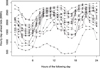 |
Figure 5 Example of the sample of the M = 20 upcoming day-ahead bids for the case study. For reasons of confidentiality, the values of day-ahead bids are arbitrarily scaled. |
3.2 Design of experiments
The size MN of the sampled input data set  is too large to evaluate the function Q at each point, since an evaluation requires solving a large MILP problem which is time consuming. Therefore we aim at evaluate the function Q at some selected input points
  , for d ∈ {1, …, D}, with D ≪ MN, m
d
∈ {1, …, M} and n
d
∈ {1, …, N}. The selected points have to be well distributed in the set
, for d ∈ {1, …, D}, with D ≪ MN, m
d
∈ {1, …, M} and n
d
∈ {1, …, N}. The selected points have to be well distributed in the set  to ensure that the numerical values
  , for d ∈ {1, …, D}, give enough information about the global structure of the function Q.
The input data are strongly correlated because upcoming day-ahead bids, water inflows, and day-ahead prices have a functional structure and possibly correlations with each other. Since sampling such input data is quite challenging, the surrogate model is constructed with the following assumptions:
-
the acceptable upcoming day-ahead bids are supposed to be independent of the scenarios,
-
the water inflows and the day-ahead prices that compose the scenarios are supposed to be independent of each other,
-
the upcoming day-ahead bids, the water inflows, and the day-ahead prices are each reduced to a scalar to remove their functional structure.
After scaling, these assumptions lead to three independent inputs in [0, 1]. For the case study, the reduction of each functional input to a scalar is performed by getting the L 1-norm for upcoming day-ahead bids and water inflows and the L 2-norm for day-ahead prices (see Fig. 6), in order to be consistent with the distance used in Section 3.1. Of course, these assumptions are strong because, in practice, the effective day-ahead bids are decided with respect to the distribution of the scenarios and because a scalar cannot accurately represent a functional data. They might however be sufficient to construct an adequate surrogate model.
 |
Figure 6 Example of the scaled scalar representation of the inputs for the case study. (a) Day-ahead bids, (b) water inflows and (c) day-ahead prices. |
We propose to construct the design of experiments by the use of a 3-dimensional Latin Hypercube Sampling (LHS) with D points and optimal with respect to the maximin criterion [32]. Based on the independence assumption on the three inputs, this approach provides a set  of D points in [0, 1]3 whose empirical distribution is close to the uniform distribution on [0, 1]3. Since each input is not necessarily uniformly distributed in [0, 1] (see Fig. 6), the design of experiments is obtained by applying the empirical quantile function of each input at the associated component of every point in
  . Let
. Let  , for d ∈ {1, …, D}, denote the selected points with their functional structure. Removing some points if necessary, we may assume that the selected points are all different.
The size D of the design of experiments is arbitrary. In practice, it is chosen according to the computing power at our disposal and the complexity (degrees of freedom) of the surrogate model. For the case study, we choose D = 1000, a very large size compared to the complexity of the surrogate model (see Sect. 4) but computation time is available in the study phase.
3.3 Data set
The data set is obtained by evaluating the function Q at each point of the design of experiments. Let  for d ∈ {1, …, D}. This requires solving D-independent large MILP problems. The data set is specific to the situation at hand and it has to be computed at each new situation since the design of experiments and the function Q change from one situation to another.
The data set is split into a learning data set with indices  and a validation data set with indices
  . The choice of the ratio of the data set that is used for fitting is arbitrary. For the case study, the chosen ratio is 60%.
4 Metamodeling
In this paper, the surrogate function  is chosen among linear models. In this case, however, the structure of the function Q might not be completely represented since the function Q is piecewise linear (see Sect. 2.3).
4.1 Dimension reduction
A dimension reduction of the inputs is necessary since their initial dimension is too large for fitting a linear model with regard to the size D of the learning data set. A common approach consists of using the coefficients of the decomposition of the inputs onto an orthonormal family with a small size. Several approaches for constructing the orthornomal family are presented in the literature (wavelets, splines, principal components analysis, etc.) [20, 33–36]. For the case study, numerical tests, which are not presented in this paper, show that Principal Components Analysis (PCA) provides the best compromise between the reduction error and the size of the family. As PCA is data-driven, the dimension reduction is described for the case study defined in Section 2.1.
Since upcoming day-ahead bids, water inflows, and day-ahead prices are assumed to be independent of each other in constructing the surrogate model, PCA is separately applied to each of the three inputs. The values of each input are centered to ensure that PCA is based on explained variance, but they are not scaled to preserve the functional structure of the inputs. If the inputs were not assumed to be independent of each other, then the orthonormal family should have been common for the three inputs. Moreover, some values of water inflows (respectively day-ahead prices) are redundant since they are not defined with time steps of duration δt = 10 min but with half-hourly (respectively hourly) time steps.
The redundant values are removed before applying PCA.
Let  denote the linear mapping that gives the coefficients of the decomposition of upcoming day-ahead bids onto the orthonormal family composed of the K1 first principal components in decreasing order of their explained variance (K1 ∈ {1, …, 24}). Let
  ) (respectively
  )) denote the similar linear mapping for water inflows (respectively day-ahead prices) after removing redundant values, with K21 ∈ {1, …, 6 × 120} (respectively K22 ∈ {1, …, 48}). Then let
  , with K2 = K21 + K22, be the linear mapping defined by concatenating ϕ21 and ϕ22, i.e.,
For the case study, K1, K21 and K22 are chosen to be the minimal number of principal components such that the cumulative explained variance is greater than 95% of the total explained variance (see Fig. 7). The threshold of 95% is arbitrary. We get K1 = 6, K21 = 7 and K22 = 13 (K2 = 7 + 13 = 20).
 |
Figure 7 Cumulative explained variance as a function of the selected number of principal components in decreasing order of their explained variance. The horizontal dashed lines represent the threshold of 95% cumulative explained variance. (a) Day-ahead bids, (b) water inflows and (c) day-ahead prices. |
4.2 Fitting
The linear model  is defined by
 where
where  ,
,  and
and  are the coefficients of the linear regression (least squares problem solved by the QR decomposition method) on the learning data set defined by the indices
  after dimension reduction of the inputs, and the superscript ⊤ stands for the transpose operator.
4.3 Validation criteria
The quality of the linear model  is assessed by its prediction errors on the validation data set defined by the indices
  . Prediction errors are evaluated on individual total revenues (see Eq. (6)) by two scores:
-
the predictivity coefficient Q2, i.e., the coefficient of determination computed on the validation data set by
![Mathematical equation: $$ {\mathrm{Q}}^2=\enspace 1\enspace -\frac{{\sum }_{d\in {\mathcal{D}}_v}^{}|{Q}_d-{\widehat{Q}}_d|}{{\sum }_{d\in {\mathcal{D}}_v}^{}|{Q}_d-{\bar{Q}}_{}|}\in \enspace \left(-\mathrm{\infty },\enspace 1\right],\hspace{0.5em}\mathrm{with}\hspace{0.5em}\bar{Q}\enspace =\enspace \frac{1}{|{\mathcal{D}}_v|}\sum_{d\in {\mathcal{D}}_v}{Q}_d\in \mathbb{R}, $$](/articles/stet/full_html/2023/01/stet20220096/stet20220096-eq85.gif) where
where  , for
, for  , are the values of the surrogate model on the validation data set.
-
the mean absolute error on the validation data set of the normalized total revenues with respect to the total revenues of the deterministic optimal solution
 of the problem in equation (2), i.e.,
 It should be noted that the two scores can be evaluated by cross-validation instead of using a validation data set, especially if the size D of the data set is small.
4.4 Results
The results of the case study are presented in Figure 8. The predictivity coefficient is Q2 = 0.9813, which is above the arbitrary threshold of 0.95 used for the case study. The mean absolute error of the normalized total revenues is MAE = 0.39%, which is below the relative MIP gap of 2% used for the case study. It turns out that the linear model is quite relevant to the case study. Thus the piecewise linear function  )] is reasonably linear on the set
  of the sampled day-ahead bids.
 |
Figure 8 Prediction errors computed on the validation data set for the case study. |
5 Discussion
The stochastic optimization problem in equation (3) is solved with the proposed methodology and compared to the deterministic optimization problem in equation (2) for the case study. We recall that the truly optimal solution of the stochastic optimization problem in equation (3) is not accessible with the CPLEX MIP solver and the computing power at our disposal (4 cores, 3.8 GHz, and 16 Go of RAM).
5.1 Computation time
For operational use in our case, the total computation time of solving the stochastic optimization problem has to be less than 3 times that of solving the deterministic optimization problem. The total computation time is composed of that of the pre-processing step and that of solving the MILP problem in equation (7).
The computation time of the pre-processing step is due to that of evaluating the optimal value function Q on the design of experiments since the computation time of discretizing the day-ahead bids and that of fitting the linear surrogate model  are negligible. Let τ
d
∈ ℝ+, for d ∈ {1, …, D}, denote the computation time of evaluating the optimal value
are negligible. Let τ
d
∈ ℝ+, for d ∈ {1, …, D}, denote the computation time of evaluating the optimal value  over that of solving the deterministic MILP problem in equation (2). Their distribution for the case study is presented in Figure 9. On average, evaluating the optimal value function Q at a point in the design of experiments requires a computation time 39.41% greater than that of the deterministic solution (reference value of τdet = 1):
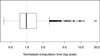 |
Figure 9 Boxplot of the normalized computation time of evaluating the optimal value function of the second stage at every point of the design of experiments for the case study. |
We also observe that some evaluations of the optimal value function Q require extreme computation time up to almost 20 times greater than that of the deterministic solution:
If the values Q
d
, for d ∈ {1, …, D}, of the data set can all be computed in parallel for the case study (i.e., unlimited access to parallel computing), then the normalized total computation time of the preprocessing step is around 20 times greater than the computation time of solving the deterministic problem in equation (2). Once the surrogate model  is fitted, the normalized computation time of solving the MILP problem in equation (7) is τopti = 1.0547, i.e., only 5.47% higher than the computation time of solving the deterministic problem in equation (2). Therefore the normalized total computation time for the case study,
 is largely determined by the computation time of the pre-processing step and it is too large for operational use (far above the acceptable threshold of 3 for our case).
The computation time of the pre-processing step can however be improved by stopping the calculation of the evaluation of the optimal value function Q if it exceeds an acceptable time limit (a normalized time limit of around 2 for our case). The extreme points of the design of experiments are then removed, but on the other hand, this process may subsequently have an impact on the quality of the surrogate model. Moreover, with limited access to parallel computing of n
t
∈ ℕ cores, the normalized computation time of the pre-processing step is estimated on average by The number D of points in the design of experiments has then to be carefully chosen so that the computation time of the pre-processing step is below an acceptable time limit (a normalized time limit of around 2 for our case). However, reducing the number D of points in the design of experiments may require reducing the dimension of the inputs, and it also may subsequently have an impact on the quality of the surrogate model.
To improve computation time, the pre-processing step could be performed offline in advance, with data available at a former situation (e.g., a couple of hours beforehand), to update the surrogate model at regular intervals. Only the MILP problem in equation (7) would be solved during the operational process with the last updated surrogate model. The total computation time would then consist only of τopti, the same order of magnitude as for the deterministic model.
5.2 Quality of the stochastic solution
Let  and
and  denote the upcoming day-ahead bids for respectively the deterministic optimal solution
  of the problem in equation (2) and the stochastic optimal solution
  of the problem in equation (7). They are presented in Figure 10 in comparison with the set
  of day-ahead bids obtained in Section 3.1. We observe that bdet and bsto are globally similar. They are at the edge of the lower boundary of the region delimited by the set
  , even outside during the 6 first hours.
 |
Figure 10 Upcoming day-ahead bids obtained for the case study from the deterministic solution (in blue) and the stochastic solution (in red) in comparison with the sample |

The quality of the surrogate model  is evaluated on
  and
and  with the same scores as in Section 4.3. The results are presented in Figure 11 for the case study in comparison with the results obtained on the validation data set in Section 4.4. We observe that the quality of the surrogate model
  is acceptable with the day-ahead bids bdet and bsto (predictivity coefficient Q2 above 0.95 and mean absolute error below 2%), even if it is slightly lower than with the discretized day-ahead bids in
  . Thus the approximate mapping
 ![Mathematical equation: $ \widehat{\mathcal{E}}:\enspace {b}_0\in {\mathcal{B}}_0\mathbf{\mapsto} \mathbb{E}[\widehat{Q}({b}_0,\widehat{\mathrm{\Xi }})]$](/articles/stet/full_html/2023/01/stet20220096/stet20220096-eq110.gif) does not significantly over-estimate the mapping
does not significantly over-estimate the mapping ![Mathematical equation: $ \mathcal{E}:\enspace {b}_0\in {\mathcal{B}}_0\mathbf{\mapsto} \mathbb{E}[Q({b}_0,\widehat{\mathrm{\Xi }})]$](/articles/stet/full_html/2023/01/stet20220096/stet20220096-eq111.gif) around the optimal region of the optimization problem. There is no guarantee, however, that the approximate mapping
around the optimal region of the optimization problem. There is no guarantee, however, that the approximate mapping  does not significantly under-estimate the mapping
  on
on  , which could misleadingly force the optimal region to be inside
  .
.
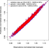 |
Figure 11 Prediction errors computed on the upcoming day-ahead bids of the deterministic solution (in blue) and the stochastic solution (in red) for the case study. |
The similarities between  and
and  may be a sign that the deterministic solution
  and the stochastic solution
  are similar. For verification, the stochastic objective function is evaluated at the deterministic solution and the deterministic objective function is evaluated at the stochastic solution. For the case study, we obtain
![Mathematical equation: $$ \frac{{\alpha }_0f\left({\mathbf{x}}_{\mathrm{det}}^{\mathbf{*}},{\xi }_0\right)+(1-{\alpha }_0)\mathbb{E}[Q({b}_{\mathrm{det}},\widehat{\mathrm{\Xi }})]}{{\alpha }_0f\left({\mathbf{x}}_{\mathrm{sto}}^{\mathbf{*}},{\xi }_0\right)+(1-{\alpha }_0)\mathbb{E}[Q({b}_{\mathrm{sto}},\widehat{\mathrm{\Xi }})]}=\enspace 1.0047\hspace{0.5em}\mathrm{and}\hspace{1em}\frac{f\left({\mathbf{x}}_{\mathrm{det}}^{\mathbf{*}},{\xi }_0\right)}{f\left({\mathbf{x}}_{\mathrm{sto}}^{\mathbf{*}},{\xi }_0\right)}=0.9933, $$](/articles/stet/full_html/2023/01/stet20220096/stet20220096-eq120.gif) so, with respect to the relative MIP gap of 2%, the deterministic solution
so, with respect to the relative MIP gap of 2%, the deterministic solution  also optimal for the stochastic optimization problem and the stochastic solution
  is also optimal for the deterministic optimization problem. For the case study, the differences between the deterministic and stochastic objective functions are then insignificant with respect to the relative MIP gap of 2%. This is due to the fact that the mapping
 ![Mathematical equation: $ \mathcal{E}:\enspace {b}_0\in {\mathcal{B}}_0\mathbf{\mapsto} [Q({b}_0,\widehat{\mathrm{\Xi }})]$](/articles/stet/full_html/2023/01/stet20220096/stet20220096-eq124.gif) is globally constant, so independent of the decision variable, as illustrated in Figure 12.
is globally constant, so independent of the decision variable, as illustrated in Figure 12.
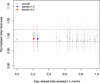 |
Figure 12 Boxplots of the normalized total revenues |

6 Conclusion
The stochastic framework of the short-term production planning of a run-of-river hydropower cascade takes into account uncertainty in forecasting water inflows and electricity prices. The problem is formulated as a mixed-integer linear two-stage stochastic dynamic programming problem. Solving this problem with a classical decomposition approach, such as an L-shaped algorithm, would require a linear relaxation of the problem and an iterative algorithm. Instead, we evaluate the feasibility of using supervised learning during a pre-processing step of the optimization. The optimal value of the second stage is replaced by a linear model so that the stochastic optimization problem becomes a tractable mixed-integer linear programming problem.
The proposed methodology is mainly based on constructing a learning data set from historically effective day-ahead bids and on reducing the dimension of the functional inputs. Validation results for one simplified case study are encouraging but the methodology needs to be improved to be compatible with the time limit of the operational process. Further results on other case studies are needed to draw general conclusions since the optimization problem is quite sensitive to the situation of the studied hydropower cascade.
The linear model could be replaced by a piecewise linear model to account for the structure of the second stage value function while keeping a mixed-integer programming formulation of the optimization problem. Moreover, in the same spirit of decomposition algorithms for solving a two-stage stochastic programming problem, metamodeling could be used within an incremental optimization procedure in which the surrogate model would be improved as approximate optimal solutions are added to the data set at each iteration, starting from a very small data set. However, it seems more appealing to perform the pre-processing step offline in advance to update the surrogate model at regular intervals. In this way, only the approximated mixed-integer linear programming model under uncertainty, defined with the last updated surrogate model, would be solved during the operational process. The deterministic and stochastic models would then have similar computation time.
Combined with intermittent energy sources (wind and solar) and electricity storage assets (e.g., renewable hydrogen), the stochastic short-term production planning can be used not only for optimizing the hydropower cascade but also the storage assets, while compensating for imbalances caused by forecasting uncertainty on intermittent generation.
References
- Fleten S.-E., Kristoffersen T.K. (2008) Short-term hydropower production planning by stochastic programming, Comput. Oper. Res. 35, 8, 2656–2671. [CrossRef] [Google Scholar]
- Labadie J.W. (2004) Optimal operation of multireservoir systems: state-of-the-art review, J. Water Resour. Plan. Manag. 130, 2, 93–111. [CrossRef] [Google Scholar]
- Tahanan M., van Ackooij W., Frangioni A., Lacalandra F. (2015) Large-scale unit commitment under uncertainty, 4OR 13, 2, 115–171. [CrossRef] [MathSciNet] [Google Scholar]
- van Ackooij W., Danti Lopez I., Frangioni A., Lacalandra F., Tahanan M. (2018) Large-scale unit commitment under uncertainty: an updated literature survey, Ann. Oper. Res. 271, 1, 11–85. [CrossRef] [MathSciNet] [Google Scholar]
- Rahmaniani R., Crainic T.G., Gendreau M., Walter W. (2017) The benders decomposition algorithm: a literature review, Eur. J. Oper. Res. 259, 3, 801–817. [CrossRef] [MathSciNet] [Google Scholar]
- Sen S. (2005) Algorithms for stochastic mixed-integer programming models, in: Handbooks in Operations Research and Management Science, vol. 12, Elsevier, pp. 515–558. [CrossRef] [Google Scholar]
- Shapiro A. (2011) Analysis of stochastic dual dynamic programming method, Eur. J. Oper. Res. 209, 1, 63–72. [CrossRef] [Google Scholar]
- van Ackooij W., Malick J. (2016) Decomposition algorithm for large-scale two-stage unitcommitment, Ann. Oper. Res. 238, 1, 587–613. [CrossRef] [MathSciNet] [Google Scholar]
- Carpentier P.-L., Gendreau M., Bastin F. (2013) Long-term management of a hydro electric multireservoir system under uncertainty using the progressive hedging algorithm, Water Resour. Res. 49, 5, 2812–2827. [CrossRef] [Google Scholar]
- Carpentier P., Chancelier J.-P., Leclère V., Pacaud F. (2018) Stochastic decomposition applied to large-scale hydro valleys management, Eur. J. Oper. Res. 270, 3, 1086–1098. [CrossRef] [MathSciNet] [Google Scholar]
- van Ackooij W., d’Ambrosio C., Thomopulos D., Trindade R.S. (2021) Decomposition and shortest path problem formulation for solving the hydro unit commitment and scheduling in a hydro valley, Eur. J. Oper. Res. 291, 3, 935–943. [CrossRef] [MathSciNet] [Google Scholar]
- Ahmed S., Tawarmalani M., Sahinidis N.V. (2004) A finite branch-and-bound algorithm for two-stage stochastic integer programs, Math. Program. 100, 2, 355–377. [CrossRef] [MathSciNet] [Google Scholar]
- Carøe C.C., Tind J. (1998) L-shaped decomposition of two-stage stochastic programs with integer recourse, Math. Program. 83, 451–464. [CrossRef] [MathSciNet] [Google Scholar]
- Gade D., Küçükyavuz S., Sen S. (2014) Decomposition algorithms with parametric Gomory cuts for two-stage stochastic integer programs, Math. Program. 144, 1–2, 39–64. [CrossRef] [MathSciNet] [Google Scholar]
- Laporte G., Louveaux F.V. (1993) The integer L-shaped method for stochastic integer programs with complete recourse, Oper. Res. Lett. 13, 3, 133–142. [CrossRef] [MathSciNet] [Google Scholar]
- Zou J., Ahmed S., Sun X.A. (2019) Stochastic dual dynamic integer programming, Math. Program. 175, 461–502. [CrossRef] [MathSciNet] [Google Scholar]
- El Amri R., Helbert C., Zuniga M.M., Prieur C., Sinoquet D. (2020) Set inversion under functional uncertainties with joint meta-models (working paper or preprint). [Google Scholar]
- Antoniadis A., Helbert C., Prieur C., Viry L. (2012) Spatio-temporal meta modeling for west African monsoon, Environmetrics 23, 1, 24–36. [CrossRef] [MathSciNet] [Google Scholar]
- Nanty S., Helbert C., Marrel A., Pérot N., Prieur C. (2016) Sampling, metamodelling and sensitivity analysis of numerical simulators with functional stochastic inputs, SIAM/ASA J. Uncertain. Quantif. 4, 1, 636–659. [CrossRef] [MathSciNet] [Google Scholar]
- Nanty S., Helbert C., Marrel A., Pérot N., Prieur C. (2017) Uncertainty quantification for functional dependent random variables, Comput. Stat. 32, 2, 559–583. [CrossRef] [MathSciNet] [Google Scholar]
- Piron V., Bontron G., Pochat M. (2015) Operating a hydropower cascade to optimize energy management, Int. J. Hydropower Dams 22, 5. [Google Scholar]
- Bellier J., Zin I., Bontron G. (2018) Generating coherent ensemble forecasts after hydrological postprocessing: adaptations of ECC-based methods, Water Resour. Res. 54, 8, 5741–5762. [CrossRef] [Google Scholar]
- Celie S., Bontron G., Ouf D., Pont E. (2019) Apport de l’expertise dans la prévision hydro-météorologique opérationnelle, La Houille Blanche 2, 55–62. [CrossRef] [EDP Sciences] [Google Scholar]
- Blair C.E., Jeroslow R.G. (1977) The value function of a mixed integer program: I, Discrete Math. 19, 2, 121–138. [CrossRef] [MathSciNet] [Google Scholar]
- Haneveld K., Van der Vlerk M.H. (2020) Stochastic programming, Springer. [Google Scholar]
- Ralphs T.K., Hassanzadeh A. (2014) On the value function of a mixed integer linear optimization problem and an algorithm for its construction. COR@ L Technical Report 14T-004. [Google Scholar]
- Bellier J., Zin I., Siblot S., Bontron G. (2016) Probabilistic flood forecasting on the Rhone River: evaluation with ensemble and analogue-based precipitation forecasts, in: E3S Web of Conferences, vol. 7, EDP Sciences, p. 18011. [CrossRef] [EDP Sciences] [Google Scholar]
- Lorenz E.N. (1969) Atmospheric predictability as revealed by naturally occurring analogues, J. Atmos. Sci. 26, 4, 636–646. [CrossRef] [Google Scholar]
- Gneiting T., Raftery A.E. (2007) Strictly proper scoring rules, prediction, and estimation, J. Am. Stat. Assoc. 102, 477, 359–378. [CrossRef] [Google Scholar]
- Hersbach H. (2000) Decomposition of the continuous ranked probability score for ensemble prediction systems, Weather Forecast. 15, 5, 559–570. [CrossRef] [Google Scholar]
- Matheson J.E., Winkler R.L. (1976) Scoring rules for continuous probability distributions, Manag. Sci. 22, 10, 1087–1096. [CrossRef] [Google Scholar]
- Santner T.J., Williams B.J., Notz W.I., Williams B.J. (2003) The design and analysis of computer experiments, vol. 1, Springer. [CrossRef] [Google Scholar]
- De Boor C. (1978) A practical guide to splines, vol. 27, Springer-verlag, New York, p. 545. [Google Scholar]
- Jolliffe I. (2005) Principal component analysis, in: Encyclopedia of Statistics in Behavioral Science, Wiley. [Google Scholar]
- Ramsay J.O., Silverman B.W. (2002) Applied functional data analysis: methods and case studies, vol. 77, Springer. [CrossRef] [Google Scholar]
- Torrence C., Compo G.P. (1998) A practical guide to wavelet analysis, Bull. Am. Meteorol. Soc. 79, 1, 61–78. [CrossRef] [Google Scholar]
Appendix
A Examples of main constraints
This appendix introduces the main constraints that apply to a feasible solution  with respect to a generic scenario
  . Note that the feasible set
  is also defined by other more detailed and specific constraints that are not presented in this paper. We continue to use the notations introduced throughout the paper.
A.1 Hydraulic modeling
The following constraints are supposed to hold.
-
The conservation of water is written by the water balance equations
 where
where  ,
,  and
and  , for
, for  , are the values of the components related to respectively the total inflows, the total outflows and the volumes of the solution x over the time horizon computed at a specific location for each hydropower facility. If a nonpositive index for the time bucket is involved, then it refers to a past value (observation).
-
The outflows are composed of discharges and spills after water propagation, so
 where
where  and
and  , for
, for  , are the values of the components related to the flow over the time horizon through respectively the hydropower plant (discharge) and the barrage (spill) that compose each hydropower run-of-river facility. The parameters
  and
and  , for
, for , denote the time delays due to water propagation between the specific location at which the balance equation is written and the physical location of respectively the plant and the barrage. If a nonpositive index for the time bucket is involved, then it refers to a past value (observation).
-
The inflows are composed of discharges and spills from the upstream facility and intermediate water inflows (e.g., from tributaries), so
 where the parameters τUS(i−1, i) ∈ ℝ+ and τBR(i−1, i) ∈ ℝ+, for
  , denote the time delays due to water propagation between the location of respectively the plant and the barrage of the upstream facility and the specific location at which the balance equation is written. If a nonpositive index for the time bucket is involved, then it refers to a past value (observation). The inflows and outflows at i = 0 are supposed to be zero. The water inflows a ∈ ℝIT is the parameter that comes from the scenario ξ.
-
The power generations are computed from discharges, i.e.,
 where
where  , for
, for  , are the values of the components related to the power generation of the solution x at each hydropower plant over the time horizon, and
  , for
, for  , are concave piecewise mappings obtained from experience. This constraint is consistent with a mixed-integer linear formulation.
A.2 Operational requirements
Operational requirements are mainly written as bounds on the decision variables. For instance, where
where  and
and  , for
, for  are parameters. Similar notations apply for inflows, outflows, discharges, spills, and for the sum of discharges and spills at each facility.
A minimal bound is also applied on final volumes to keep enough water in the reservoirs for the days after the horizon, i.e., where
where  , for
, for  , are parameters.
A.3 Objective function
The following constraints are supposed to hold.
-
Next day-ahead bids are hourly contracts, so
 where
where is the set of the first time bucket of every hour covered by the time horizon. For the case study,
  .
.
-
The next day-ahead bids are only defined on time buckets for which the day-ahead market has not yet been closed, so
 where
where  is the set of the time buckets for which the day-ahead market has already been closed (i.e., for which the day-ahead commitments are known at present). For the case study,
  with t
b
= 72 the index of the time bucket that ends on 2014-04-26 24:00.
with t
b
= 72 the index of the time bucket that ends on 2014-04-26 24:00.
-
Imbalances are the difference between real power delivery and total commitments, so they can be estimated by
 where e
t
(x) ∈ ℝ, for
where e
t
(x) ∈ ℝ, for  , are the values of the components related to the imbalances of the solution x over the time horizon, and c(t) ∈ ℝ, for
  , are the commitments that are known at the present time (i.e., day-ahead commitments that were decided the previous day since long-term commitments are assumed to be zero).
-
The hydropower production plan complies with the next day-ahead bids, so
 where
where  and
and  , for
, for  , are respectively the minimal and maximal bounds on imbalances.
-
Positive and negative imbalances are deduced from imbalances by the following constraints that are consistent with a mixed-integer linear formulation

All Figures
|
Figure 1 CNR’s hydropower plants along the Rhône river. (a) Rhône river, (b) upper part of the Rhône river and (c) scheme of the Rhône cascade. |
| In the text | |
|
Figure 2 Example of the ensemble forecasts (grey lines) taking part in the case study, the deterministic forecasts (thick blue lines), and the observations that were known at the present time (red lines). The ensemble forecasts for water inflows and day-ahead prices have 50 members each. The vertical dashed lines represent the beginning of the time horizon on 2014-04-26 12:00 (local time). For reasons of confidentiality, the forecast values of day-ahead prices are arbitrarily scaled. (a) Water inflows from the six natural tributaries taking part in the upper Rhône river over the time horizon and (b) day-ahead electricity prices over the time horizon. |
| In the text | |
|
Figure 3 Example of the planned total power generation of a solution |
| In the text | |
|
Figure 4 The average CRPS as a function of the size M of the sample for the three comparison parameters. A minimum is attained at M = 21 with the distance based on the L 1-norm of the cumulative water inflows (second comparison parameter). |
| In the text | |
|
Figure 5 Example of the sample of the M = 20 upcoming day-ahead bids for the case study. For reasons of confidentiality, the values of day-ahead bids are arbitrarily scaled. |
| In the text | |
|
Figure 6 Example of the scaled scalar representation of the inputs for the case study. (a) Day-ahead bids, (b) water inflows and (c) day-ahead prices. |
| In the text | |
|
Figure 7 Cumulative explained variance as a function of the selected number of principal components in decreasing order of their explained variance. The horizontal dashed lines represent the threshold of 95% cumulative explained variance. (a) Day-ahead bids, (b) water inflows and (c) day-ahead prices. |
| In the text | |
|
Figure 8 Prediction errors computed on the validation data set for the case study. |
| In the text | |
|
Figure 9 Boxplot of the normalized computation time of evaluating the optimal value function of the second stage at every point of the design of experiments for the case study. |
| In the text | |
|
Figure 10 Upcoming day-ahead bids obtained for the case study from the deterministic solution (in blue) and the stochastic solution (in red) in comparison with the sample |
| In the text | |
|
Figure 11 Prediction errors computed on the upcoming day-ahead bids of the deterministic solution (in blue) and the stochastic solution (in red) for the case study. |
| In the text | |
|
Figure 12 Boxplots of the normalized total revenues |
| In the text | |
Current usage metrics show cumulative count of Article Views (full-text article views including HTML views, PDF and ePub downloads, according to the available data) and Abstracts Views on Vision4Press platform.
Data correspond to usage on the plateform after 2015. The current usage metrics is available 48-96 hours after online publication and is updated daily on week days.
Initial download of the metrics may take a while.