")
")
| Issue |
Sci. Tech. Energ. Transition
Volume 78, 2023
|
|
|---|---|---|
| Article Number | 30 | |
| Number of page(s) | 19 | |
| DOI | https://doi.org/10.2516/stet/2023023 | |
| Published online | 20 October 2023 | |
Regular Article
Carnot: a thermodynamic library for energy industries
1
IFP Energies Nouvelles, 1 et 4 Avenue de Bois-Préau, 92852 Rueil-Malmaison Cedex, France
2
IFP Energies Nouvelles, Rond-point de l’échangeur de Solaize, BP 3, Solaize 69360, France
* Corresponding author: This email address is being protected from spambots. You need JavaScript enabled to view it.
Received:
6
March
2023
Accepted:
28
August
2023
Abstract
For more than twenty years, IFP Energies Nouvelles has been developing the thermodynamic library Carnot. While devoted to the origin of the oil and gas industry, Carnot is now focused on applications related to the new technologies of energy for an industry emphasizing decarbonization and sustainability, such as CCUS, biomass, geothermal, hydrogen, or plastic and metal recycling. Carnot contains several dozens of predictive and correlative thermodynamic models, including well-established and more recent equations of state and activity coefficient models, as well as many specific models to calculate phase properties. Carnot also contains a dozen flash algorithms making possible the computation of various types of phase equilibrium, including not only two-phase and three-phase fluid equilibria but also configurations with reactive systems and with solid phases such as hydrates, wax, asphaltene, or salts. The library Carnot has a double role: first, it is a standalone toolbox for thermodynamic research and development studies. Coupled with an optimization tool, it allows to develop new thermodynamic models and to propose specific parameterizations adapted to any context. Secondly, Carnot is used as the thermodynamic engine of commercial software, such as Carbone™, Converge™, TemisFlow™, CooresFlow™ or Moldi™. Through this software, several hundreds of end-users are nowadays performing their thermodynamic calculations with Carnot. It has also been directly applied to design industrial processes such as the DMX™ process for CO2 capture, the ATOL® and BioButterFly™ solutions for bio-olefins production, and Futurol™ and BioTFuel™ for biofuels production. In this context, this article presents some significant realizations made with Carnot for both R&D and industrial applications, more specifically in the fields of CO2 capture and storage, flow assurance, chemistry, and geoscience.
Key words: Thermodynamics / Library / Energy / Equation of state / Flash algorithm
© The Author(s), published by EDP Sciences, 2023
 This is an Open Access article distributed under the terms of the Creative Commons Attribution License (https://creativecommons.org/licenses/by/4.0), which permits unrestricted use, distribution, and reproduction in any medium, provided the original work is properly cited.
1 Introduction
Over the past decades, the need for producing and storing energy efficiently has motivated the development of innovative technologies in many fields, such as geoscience, chemistry, chemical engineering, materials, flow assurance, etc. Moreover, in the past years, the fight against global warming has tended to speed up process improvements and favor the emergence of new research fields. Most of the existing and developing technologies require the use of a specific and fundamental science: thermodynamics. This science describes how matter changes with temperature, pressure, and composition. In the continuity of the 17 Sustainable Development Goals defined by the United Nations for a better world [1], the Thermodynamics and Transport Properties working party of the European Federation of Chemical Engineering identified 6 main topics in which thermodynamics plays a significant role [2]: energy efficiency, water, sustainable solvents, biosciences, novel materials, and advanced material recovery. This highlights the impressive diversity of systems to be considered, including e.g. electrolytic systems, amorphous and glassy polymers, light gases, organic solvents, metals, drugs, etc. It also emphasizes the need to cover a wide range of operating conditions, for example from extremely low temperatures in the case of cryogenic processes to very high temperatures for high-enthalpy geothermal resources. This extensive range of applications and operating conditions has led to the development of a significant number of thermodynamic models and dedicated parameter sets over the past.
At the end of the 19th century, van der Waals [3] paved the way for a modern vision of thermodynamic modeling with his first equation of state for real gases. From this pioneering work, researchers have developed several dozens of models (correlations, activity coefficient models, equations of state, …) and algorithms (in particular multiphase flash calculation) covering the important diversity of industrial contexts. During the two last decades, several commercial thermodynamic engines have been released for various purposes, like PVTSim [4], PVT Package [5], Multiflash [6], Specs [7], and Simulis Thermodynamics [8]. More recently, a number of open-source thermodynamic libraries have been developed and published, like CoolProp [9], thermo [10], phasepy [11], thermopack [12], FeOs [13], teqp [14], clapeyron.jl [15], but their content is also considerably restricted in terms of a number of models and algorithms. Their usage is restricted to research and development studies, and are not designed to be plugged into industrial software.
For more than 20 years, IFP Energies Nouvelles (IFPEN) has been developing a thermodynamic library, called Carnot. As a major research and training center in the field of energy, the areas of expertise of IFPEN are climate, environment and circular economy, renewable energies, sustainable mobility, and responsible oil and gas. The research and development made at IFPEN aim at overcoming existing scientific and technological challenges in order to develop innovative solutions for industry. All of these expertise areas require thermodynamic studies, thus requiring a flexible thermodynamic library where IFPEN researchers can develop adequate approaches, that can readily be plugged into industrial software. Therefore, Carnot now contains a significant number of thermodynamic models and algorithms. The first ones were designed for up- and downstream oil and gas applications. In the last decade, many new concepts have been added related to the new technologies of energy for a decarbonated and sustainable industry. Today, new questions emerge related to a circular economy, for example, polymer recycling and hydrometallurgy.
In addition, Carnot is designed in close collaboration between thermodynamic experts and software engineers, so that it can optimally respond to its double role. First, it is a standalone toolbox for thermodynamic research and development studies. Coupled with an optimization tool, it allows developing new thermodynamic models and proposing specific parameterizations adapted to any context. Second, it is a library that can be plugged into industrial software or process simulators to develop new technologies. Many examples will be provided in this article.
This document is structured as follows: in Section 2, the global architecture and the content of Carnot are described. The four next sections illustrate how Carnot was successfully used in various industrial contexts, like CO2 capture and storage (Sect. 3), fluid transport (Sect. 4), chemistry (Sect. 5), and geoscience (Sect. 6). The links between the use of Carnot and relevant commercial software or industrial projects will be highlighted. The last section of this article is devoted to the use of Carnot as a research and development tool for thermodynamic studies, with a focus on the development of new models in challenging fields.
2 Carnot structure and interface
Carnot is coded in C++ and contains roughly 200.000 lines of code lines. Although less user-friendly than recently interpreted languages such as Python, C++ is known to offer good computation performances and interoperability between languages as it can be wrapped within the C interface. For example, Carnot offers interfaces for languages such as Fortran (based on C procedural interface), Java, Python, and C# (using SWIG [16]). Carnot also offers a CAPE-OPEN [17] interface which is well-known in the Computer Aided Process Engineering area. We are also working on a web service/web application to match Industry 4.0 [18] new ways of working. To address these new challenges, Carnot is thread-safe, which means that it can be used in multi-threaded applications on multi-core architectures. As Carnot is implemented in C++, it can be easily built natively on Windows and Unix systems. This cross-platform building feature is handled by CMake [19] which is a scripting language that allows generating several final build environments (such as Microsoft solution for Windows system or makefile for Unix system). The non-regression tests suite is implemented using the Google test framework [20] with more than 3500 test cases that are launched every night using Jenkins continuous integration server [21]. This makes it possible to make sure that any new development does not destroy previous ones: all researchers are then prompted to create new tests whenever a new development is made (either a new model or a modification of an existing one). Before validating the code, all tests are then run, and conflicts are resolved. A new version of Carnot can only be issued when all existing tests are validated. Finally, Apache Subversion [22] is used as code source versioning. Even if Git [23] supplants the Subversion solution, we are considering that Git is a little bit more complex for business developers who are moreover used to following the Subversion paradigm. This versioning tool allows the creation of branches where researchers can develop their own model without impacting the quality of the global library. When their development is finished, and if it is decided that the work deserves to be merged within the library, the branch is merged on the trunk and potential conflicts (when the same code may have been modified by several researchers) are treated.
Carnot can be broadly split into two types of classes: the container classes and the computational classes. Among the container classes, one finds fluids and systems (collections of fluids) on the one hand, and elements on the other hand. Elements are essentially a collection of parameters. Parameters are constant numerical values. One may have unary, binary, or ternary parameters, signifying that they are associated with a single element or a combination of two, or three elements. Elements may be compounds, but they also may be groups, sites, or atoms. An element may be constructed from a series of sub-elements. This combination makes it possible to allow for many applications, such as reactive flashes (a compound is made out of atoms and will react to keep the total number of each atom type constant) or group contributions (parameters for a given compound are computed from its contributing groups). The interaction sites have been added for association models (e.g. CPA or SAFT equation of state). All elements can be labeled (solvent, solute, ion, …) thus allowing for different treatments dependent on the label. Fluids and systems are associated with a thermodynamic state: they contain, in addition to a composition, a number of properties and a physical state. Computations are performed on the fluids or on systems. The second type of class are computational ones. They also can be distinguished into two categories. The first one is the Operations, whose aim is to transform an input fluid into another fluid or set of fluids. A flash calculation is a representative example of an Operation. The second category of computation is Models, which consist in calculating a property of a given fluid. Throughout its existence, a significant number of Models and Operations have been implemented in Carnot, making it probably one of the most complete existing thermodynamic toolkits. The list of features currently available in Carnot is given in Tables 1 and 2.
List of models available in Carnot (version 10).
List of operations available in Carnot.
An interesting feature that has been implemented is the concept of thermodynamic method which contrasts the thermodynamic model. A method is nothing but a combination of models that are assigned to different property calculations and different fluid types. The use of this concept makes it possible to construct virtually any combination of models and sub-models for any thermodynamic property (homogeneous or heterogeneous approaches, symmetric or asymmetric ones, …).
3 Carnot for CO2 capture and storage
CO2 Capture and Storage (CCS) is one of the most promising ways to reduce greenhouse gas emissions. According to the International Energy Agency (IEA), 35 CO2 capture facilities are today collecting more than 40 Mt of CO2 annually, and this amount will drastically increase in the near future since more than 300 CCS projects are currently at various stages of development [24].
3.1 CO2 capture
The 3D project (DMX™ Demonstration in Dunkirk) [25] is a promising capture technology aiming at capturing efficiently CO2 with a significant reduction of energy consumption. This project is currently at the stage of industrial demonstration. The thermodynamic model is essential for the dimensioning of the process, in particular the unit of acid gas absorption by the solvent and the unit of solvent regeneration. Due to a coupling between chemical reactions in the liquid phase and phase equilibrium, it is also necessary to use a reactive flash algorithm. It is possible to treat this type of problem in two ways: one is to use an algorithm that explicitly takes into account the stoichiometries of the reactions and the other uses a global minimization approach of the Gibbs free energy of the system [26]. Both approaches are available in Carnot and give the same results. The first alternative is more efficient in terms of computation time and stability when few reactions occur. It is therefore only suitable for a well-defined set of reactions. The second way, on the contrary, is fully generalizable. The value of either approach depends on the number of compounds to be processed and the number of reactions that take place. If only a few reactions are to be considered, then the stoichiometric approach may be more efficient in terms of computation time and stability. The non-idealities can be treated by either equations of state or activity coefficient models. In Carnot, several activity coefficient models for such systems are available, such as Deshmukh and Mather [27] and e-NRTL [28].
Figure 1 shows an example of results in terms of speciation profiles in a DMX solvent solution. These results have been obtained with Carnot using a stoichiometric reactive flash algorithm coupled with the thermodynamic model of Deshmukh and Mather.
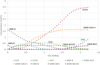 |
Fig. 1 Concentration profiles of a DMX solution with CO2. The DMX solvent is composed of water and two amines: DMX-A & DMX-B. Calculations done with the Deshmukh and Mather model in Carnot. |
This speciation allows reproducing the different absorption isotherms as shown in Figure 2.
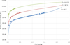 |
Fig. 2 Isotherms of CO2 capture by a DMX-A solution. Symbols are experimental data and lines are model results. Calculations done with the Deshmukh and Mather model in Carnot. |
Finally, Tsanas et al. [29] extended these calculations to liquid–liquid reactive equilibrium simulations. They show that it is possible to use rigorous thermodynamic tools to reproduce, not only liquid–vapor but also liquid–liquid equilibria with e-NRTL, using a reactive flash, by direct minimization of the system Gibbs free energy.
3.2 CO2 storage
When dealing with CO2 storage in aquifers or in depleted reservoirs, a major concern is what quantity of CO2 can be dissolved in the brine. An accurate calculation is required to correctly evaluate the storage capacity of a geological formation and to predict the possible interactions with the surrounding rock. To this end, Carnot has been embedded in the industrial software CooresFlow™ [30], whose aim is to simulate CO2 injection and storage with a multi-physics and multi-scale approach. A recent study with this simulation software [31] used a diphasic TP flash with the Soreide and Whitson model [32] (S&W) to predict the CO2 solubility in brines for various temperatures, pressures, and salinities. Note that the S&W model implementation in Carnot uses a revised binary interaction parameter between CO2 and brines parameterized on recent experimental data [33]. Figure 3 shows a comparison between experiments and results obtained with Carnot. A very good agreement is found (average deviation around 5%) on the investigated temperature, pressure, and salinity ranges (323–423 K, 1–400 bar, 0–6 mol/kg).
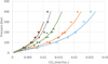 |
Fig. 3 CO2 solubility in pure water and in brines (NaCl) at 373.15 K. Symbols: experiments [33–36] (open squares: in pure water; triangles: salinity = 1 mol/kg; diamonds: salinity = 3 mol/kg; squares: salinity = 5 mol/kg; circles: salinity = 6 mol/kg). Lines: calculation with the S&W model in Carnot. |
4 Carnot for fluid transport
4.1 Gas permeation
The use of flexible pipes for fluid transport has many advantages [37]. Their construction is however very complex, as they need to resist high internal pressures and strong mechanical constraints, as well as be resistant over time. In the context of a long-standing collaboration between IFPEN and TechnipFMC, a software, called Moldi™, has been developed [38] for describing the radial permeation of gases through the different polymer sheaths that make up the pipe. This software is interfaced with Carnot and uses TP and TV flashes to evaluate whether water may possibly condense in the annular space between an inner and an outer polymer layer. Condensation is problematic because it may lead to corrosion of the metallic material that assures the mechanical strength of the pipe. Recently, the permeation equation has been adapted to replace Fick’s law with an augmented diffusion law that takes into account fugacities [39]. The CPA equation of state [40] is used in this context for computing both two- and three-phase equilibria of systems containing methane, CO2, water, and other minor compounds. The Carnot isochoric (TV) flash was specifically adapted to this application. Further work on this topic is progressing with the objective of using PC-SAFT [41] within the polymer material.
4.2 Asphaltene flocculation
Both qualitative and quantitative approaches for asphaltene precipitation are available in Carnot. One of the most-known qualitative models is the de Boer method [42], which allows screening crude oils on their asphaltene deposit tendency. By correlating crude properties, e.g., solubility parameter, molar volume, and asphaltene solubility in oil, with the density of the crude at in situ conditions, this model provides an asphaltene supersaturation plot (or de Boer plot), showing the risk level of asphaltene flocculation during production [42].
An example of the de Boer plot calculated with Carnot is given in Figure 4, which shows the difference between the reservoir pressure and the bubble pressure versus the in-situ density of the oil sample. There are three distinct zones, in which the fluid is considered unstable (Region A) with severe problems, slightly unstable (Region B) with moderate risks, and stable (Region C) with negligible asphaltene precipitation [42]. The example of fluid C1 from [43] is located in the unstable region.
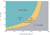 |
Fig. 4 The de Boer plot illustrating (Pr–Pb = difference between the reservoir pressure and the bubble pressure of the fluid) versus the fluid density. The red point corresponds to the fluid C1 from [43]. |
The quantitative approach is a compositional model that allows calculating the amount of asphaltenes precipitated in given temperature and pressure conditions. The compositional asphaltene model in Carnot considers the flocculation of asphaltenes as liquid–liquid demixing [44–47]. It results in three-phase liquid–liquid–vapor phase equilibrium calculations. Thermodynamic phase equilibria of the system can be modeled by two approaches, both based on group contribution methods. The first approach involves the Peng–Robinson equation of state (1976) associated with the group contribution mixing law of Abdoul–Péneloux [48, 49] while the second one uses the PPR78 model [50, 51].
The calculation results obtained with the asphaltene compositional Abdoul–Péneloux model on the fluid C1 from Figure 4, are shown in Figure 5. The effect of temperature on saturation pressure Psat and Upper Asphaltene Onset Pressure (UAOP), the pressure where asphaltenes start precipitating, is examined (Fig. 5a). The results are in very good agreement with experimental data. Figure 5b depicts the effect of pressure on the quantity of precipitated asphaltenes at different temperatures. It is known that the amount of asphaltene deposit reaches a maximum value at saturation pressure Psat [44, 45, 52]. This phenomenon is well reproduced by Carnot. It is noticed that the Upper Onset Pressures (UAOP) range from 350 to 400 bar for the considered temperatures, as also illustrated in Figure 5a.
 |
Fig. 5 Bubble pressure and asphaltene precipitation upper onset pressure (UAOP) as function of the temperature for the reservoir fluid C1 [43] (a) and weight fraction of precipitated asphaltenes (b). |
Both qualitative and quantitative asphaltene models in Carnot are embedded in the industrial software Carbone™ [53], alongside a parameter regression workflow to fit experimental data for the quantitative model.
4.3 Hydrate formation
Gas hydrate formation, even though it is something that has negative consequences in the petroleum and gas processing industry, also has the potential for numerous positive applications such as CO2 capture and sequestration, gas storage, water desalination/treatment technology, etc [54]. Hence, predicting hydrate equilibrium pressure, temperature, and composition as well as hydrate phase properties are of great interest.
In Carnot, a hydrate module to simulate hydrate formation/dissociation conditions has been implemented. In this module, the hydrate phase is simulated with the van der Waals et Platteeuw model [55] using the Kihara potential approach. The fluid phase is modeled with the CPA equation of state [40]. Coupling these models allows the user to compute several essential pieces of information such as:
-
Diphasic and triphasic equilibrium temperature/pressure (in the presence of the water phase: H-V-Lw and without liquid water: H-V),
-
Hydrate composition,
-
Effects of thermodynamic inhibitors on the shift of the equilibrium curve,
-
Stability region of hydrates without or with inhibitors.
The hydrate module has been validated with a wide range of experimental data. An example of predictions for three simple hydrates as well as for two natural gases is illustrated in Figure 6. This hydrate equilibrium calculation module is embedded in the commercial software Carbone™ [53].
In addition to hydrate formation/dissociation calculations, specific models that allow the determination of hydrate properties such as lattice parameter, density, entropy, enthalpy, and heat capacity are available in Carnot. Figure 7 gives an illustration of the lattice parameter of CO2 hydrates at different temperatures and ambient pressure. The results obtained with Carnot are based on the correlation proposed by Vins et al. [61] and are compared to some available experimental data.
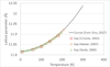 |
Fig. 7 CO2 hydrate lattice parameter calculated with Carnot and compared with experimental data [61–64]. |
4.4 CFD computations
In the context of internal combustion engine modeling, high-speed computational fluid dynamic is used to describe the fuel injection. As the fuel evaporates, there is a need to describe the fluid properties, which include internal energy, enthalpy, but also the speed of sound. Carnot was used for this purpose with cubic equations of state for hydrocarbon mixtures [65] or more advanced equations of state such as CPA or SAFT for mixtures including associative compounds. When the fuel is composed of a mixture, the direct use of Carnot in the fluid dynamics simulator becomes very cumbersome in computation time. It was found necessary to preprocess the thermodynamic computation by generating a large table that is interpolated during the actual calculations [66]. An alternative approach to decrease the computation time has been investigated separately using artificial neural networks [67]. We believe that such coupling of a true thermodynamic calculation with machine learning may be a very efficient way to enlarge the scope of applications of conventional thermodynamic methods.
5 Carnot for chemistry
5.1 Product characterization (new generation of fuel)
For the formulation of the new generation of fuels, and more specifically those produced from biomass, it is of primary importance to evaluate their evaporation behavior in order to design the appropriate engine injectors. The main objective is to limit the formation of deposits that could clog the combustion organs and cause particle emissions that must be reduced as much as possible. In this context, in situ imaging is a powerful tool to characterize the behavior of the fluid in the various combustion organs, and optical diagnostic tools allowing the visualization of film and deposit formation in enclosures have been developed [68]. The idea is to include optical tracers in the fuel that will evaporate preferentially depending on the type of compounds. It is thus possible to identify tracers that will characterize the evaporation of light cuts (volatile compounds) and others that correspond to heavier compounds. The figure below illustrates this methodology with the distillation curve of a fuel (blue curves) and the evaporation curves of optical tracers which are characteristic of a temperature range. The choice of tracers in adequacy with the distillation curve of the fuel is performed using thermodynamic calculations. The distillation curve is represented as a succession of saturation temperature calculations at given vapor fraction by removing at each step the totality of the existing vapor phase. The modeling of the phase equilibria is done with Predictive SRK (PSRK) [69]. These calculations are done with an in-house software embedding Carnot. Figure 8 compares the distillation curves of a biofuel (represented by a surrogate) and the calculation model. The curves of different optical tracers are also included, making it possible to quantify the fuel evaporation.
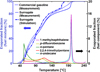 |
Fig. 8 Distillation curves and tracer profiles of a biofuel. From [68]. All simulations are performed with Carnot. |
5.2 Bio-sourced products
The chemical industry must address the challenge of producing more sustainable products with a lower carbon footprint. Such a challenge paved the way for bio-sourced product development. In the field of petrochemistry, it often means using bioethanol (produced from biomass) instead of fossil ethanol (produced from oil). Recently, new chemical processes have been released to produce bio-based olefins (ethylene, butene, butadiene) from bioethanol, like the ATOL® and the Biobutterfly™ technologies offered by the company Axens [70]. In the same idea, new technologies have been developed to produce biofuels from lignocellulosic biomass (second-generation advanced biofuels), such as the BioTfuel® technology for renewable diesel and sustainable jet fuel [71].
To develop and design these new technologies, Carnot has been used as the thermodynamic engine for the process simulators. More specifically, triphasic TP flashes (between a gas phase, an aqueous phase, and an organic phase), used in association with the SRK-Twu model (SRK equation of state with the alpha function and the mixing rules of Twu [72]) are performed to calculate separation columns along the process. Figure 9 shows an example of a heteroazeotropic diagram calculated for the binary mixture water + 1-butanol, a key-binary in the bio-butanol dehydration process in bio-butene. The alpha function parameters for pure 1-butanol and pure water have been adjusted to match experimental vapor pressures and liquid heat capacities:![Mathematical equation: $$ {\alpha }_{1-\mathrm{butanol}}={\mathrm{Tr}}^{0.163(3.0007-1)}\mathrm{exp}\left[3.217\left(1-{\mathrm{Tr}}^{0.4891}\right)\right], $$](/articles/stet/full_html/2023/01/stet20230034/stet20230034-eq1.gif)
![Mathematical equation: $$ {\alpha }_{\mathrm{water}}={\mathrm{Tr}}^{2.07355(0.87713-1)}\mathrm{exp}\left[0.4432\left(1-{\mathrm{Tr}}^{1.8188}\right)\right], $$](/articles/stet/full_html/2023/01/stet20230034/stet20230034-eq2.gif) where Tr is the reduced temperature of the component (Tr = T/Tc where Tc is the critical temperature of the component).
where Tr is the reduced temperature of the component (Tr = T/Tc where Tc is the critical temperature of the component).
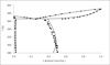 |
Fig. 9 Phase diagram of the binary mixture water + 1-butanol at atmospheric pressure. Symbols: experimental data. Lines: SRK-Twu model (Carnot). |
Four empirical parameters involved in the Twu mixing rules (asymmetric temperature-dependent binary interaction parameters) have been fitted to match simultaneously liquid–liquid (LLE) and liquid–vapor (VLE) data:

This parameterization allows good accuracy for the whole phase diagram, with a single parameter set for both VLE and LLE.
6 Carnot for geosciences
6.1 Geothermal
Salt deposition, usually referred to as scaling, is a serious problem often observed in geothermal plants. Scale formation occurs from the underground porous media up to the surface through pipelines and other production equipment and facilities. The main reason behind mineral precipitation is super-saturation, which happens when a solution contains dissolved materials at higher concentrations than their equilibrium concentration. Super-saturation can occur in water due to changes in temperature, pressure, pH, and acid gases (CO2 and H2S) partial pressure [73–75]. It probably also occurs by mixing two solutions with different speciations that interact chemically. As an example, scale precipitation can be seen during seawater flooding or brine water injection. In this case, seawater typically containing high concentrations of  will meet formation water from an underlying water zone, with high concentrations of Ca2+, Ba2+, and Sr2+. Mixing these waters causes precipitation of calcium, barium, and strontium sulfates.
It is then convenient to have information about the risk of salt precipitation under operating conditions. For this purpose, two different modeling approaches are possible with Carnot. The first approach involves a qualitative estimation via the degree of super-saturation of salts, also known as the saturation index, that allows for identifying which salts can possibly precipitate depending on input conditions. The qualitative nature of this approach relies on the fact that the amount of salt solids is not quantitatively determined. The second approach calculates in a quantitative manner the amount of mineral precipitation as solid salts. Both qualitative and quantitative approaches are available in Carnot, and embedded in the commercial software Carbone™ [53]. The seven following salts are considered in this module: sodium chloride (NaCl), calcium sulfate (CaSO4), barium sulfate (BaSO4), strontium sulfate (SrSO4), calcium carbonate (CaCO3), iron carbonate (FeCO3), iron sulfide (FeS).
The saturation index SI of a salt MX, that dissociates into cation M and anion X, is defined as follows: where aM and aX are the activity of salt ions in the aqueous phase and
  is the salt solubility product. Negative SI implies sub-saturation, the salt will not precipitate. SI equal to zero implies saturation and the solid starts to form, while SI is positive for salts likely to precipitate.
According to the context, the aqueous phase may also contain dissolved acid gases like CO2 and H2S. In our approaches, the thermodynamic phase equilibrium is evaluated by reactive flash calculations based on the minimization of Gibbs free energy under mass balance and electroneutrality constraints. Classical equations of state (PR or SRK) are used to account for the non-ideality of hydrocarbon phases, while the activity of ionic compounds is calculated by Pitzer’s model [76–78]. The saturation indexes of different salts are then calculated from the activity of corresponding ions via the above equation. For the quantitative approach, additional solid phases should be considered in the reactive equilibrium calculation and the quantity of precipitated solid salt is then determined.
Figure 10 illustrates an example of a saturation index diagram (also known as pre-scaling tendencies plot) calculated with Carnot, showing the temperature dependence of SI of different salts at a fixed pressure of 10 bar. The composition of the water used for this calculation is provided in Table 3.
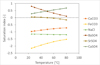 |
Fig. 10 Saturation index of various salts versus temperature at pressure of 10 bar. The composition of the water is in Table 3. |
Compositional analysis of the water used for the saturation index calculation.
Another example can be found in Figure 11 that plots the simulated results of scale precipitation when mixing formation water and seawater at 25 °C and 1 bar. The detailed composition of these two aqueous solutions can be found in [79]. The water is assumed to be in equilibrium with a gas containing 3.6 mol% CO2 as in [80]. The results obtained with Carnot (solid lines with markers) are found in very good agreement with the reference results provided by Pedersen et al. [80] (dashed lines in Fig. 11).
 |
Fig. 11 Simulated results of scale deposit when mixing formation and seawater at 25 °C and 1 bar: saturation index (a) and quantity of precipitated salts (b) versus volume fraction of seawater. |
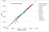 |
Fig. 12 Comparison between experimental data [81–94] and predicted silica solubilities in pure water from 20 °C to 900 °C and pressure up to 20,000 bar. |
In the special case of high pressure precipitation of compounds with very low solubilities in a given solvent, it is possible to treat the liquid–solid equilibrium with a density approach. In this approach, the apparent mass action law of dissolution can be simply correlated as a function of temperature and solvent density. The effect of pressure on the apparent solubility constant is then taken into account through the solvent density correlation. A typical example in the context of deep geothermal energy concerns silica deposition:
Mass-action relation is applied to this equilibrium and leads to: where
where  is the activity of silica in water. As the solubility is low, we can assume that activity is equal to the molality of silica (ideal solution) and then:
 where
where  is the silica molality (mol. of silica by kg of water). The density model is based on the empirical observations that the solubility constant is related to the temperature and the density of pure water. Thus, it is possible to describe the solubility limit of silica over a wide range of temperature and pressure.
The interest of such an approach is that it is possible to treat the solubility of trace compounds in complex brines by simply knowing the density of these brines and some experimental data allowing adjustment of the correlation of the mass action law. Such an approach has been applied with Carnot using the electrolyte CPA equation of state to model the brine density for a large range of temperatures and pressures. It allowed us to determine the saturation limits of trace compounds for a deep geothermal context, in order to limit the risks of salt precipitation for the process along the pressure-temperature profile.
6.2 Gas storage in caverns or aquifers
The production of renewable energies like solar or wind will drastically increase in the near future as a response to climate change issues. As these energies are by nature intermittent, they must be stored during high-production phases and released when the demand is important. A solution would consist in converting the produced electricity into an energy carrier like hydrogen or compressed air (CAES), which may be stored underground, more specifically in a salt cavern whose permeability is very low [95, 96].
In this context, Carnot has been used in preliminary projects with industrial partners to evaluate the solubility of both hydrogen and air in saturated brines, and the moisture of the gas produced during the withdrawal phases [97, 98]. Diphasic TP flash calculations have been performed using an electrolyte version of the PC-SAFT equation of state. The need of using such an advanced equation of state is motivated by two constraints: a high-pressure operating condition, and a salinity close to saturation. This model has been first parameterized to reproduce accurately the mean ionic activity coefficient of the Na+ and Cl− ions in water on the whole concentration range. Binary interaction parameters between light gases (H2, N2, O2) and ions have then been fitted to reproduce solubility data. Figure 13 shows a comparison of hydrogen in salted water between the calculated values with Carnot, and experimental data not used in the parameterization database, to evaluate the predictivity of the model. A very good agreement is achieved, with an average deviation of less than 5%, close to the experimental uncertainty.
 |
Fig. 13 Predictions of hydrogen solubility in salted water at 323 K (left) and 373 K (right). Lines: e-PPC-SAFT model. Symbols: experimental data not used in the parameterization database [99]. Orange diamonds: 1 mol/kg. Green triangles: 3 mol/kg. Blue circles: 5 mol/kg. |
6.3 Reservoir and basin modeling
Basin modeling consists in predicting the reservoir physics involved in fluids accumulation through geological times. Generally, the analysis spans from the burial of the source rock to the hydrocarbon generation, migration, trapping, accumulation, and further basin development [100]. Precisely, simultaneous geological phenomena are numerically solved to describe reservoir reconstruction, such as sediment compaction, pressure generation, heat transfer, and fluid flow behavior.
These complex calculations are made by currently available 3D basin exploration software. Since 2006, IFPEN has been developing this type of modeling tool, with a commercial solution named TemisFlow™ [101, 102]. This software allows solving a complex system of non-linear partial differential equations, representing Darcy’s and compaction laws, heat balances, and material balances of solid and fluid phases in the reservoir [100, 103]. Currently, the software allows calculating accumulated volumes and predicting the migration of multiphasic fluids (vapor, organic liquid, and water), being supported by the thermodynamic library Carnot.
One of the complexities of the modeling of multiphase fluid migration is the determination of phase transition conditions [104, 105]. Along the fluid migration path, fluid phases can be formed or dissolved after changes in pressure, temperature, and composition. These transitions can affect the flow regime, caused by differences in phase velocity. Additionally, fluid compositions can change after a phase transition (formation or dissolution), impacting the assessment of fluid quality. For that reason, a robust phase identification procedure is necessary to identify the phases in equilibria and their properties.
In this context, Carnot is used either to perform multiphase flash calculations at defined pressure and temperature along the reservoir evolution or to determine the fluid thermodynamic state. The flash calculation handles rigorous compositional modeling of the reservoir fluids, determining phase splitting up to three phases, i.e., vapor, liquid, and/or aqueous, together with their respective compositions. The phase identification needed for subsequent use in reservoir modeling, such as Darcy’s law calculations, is also performed within Carnot.
Carnot includes different phase identification criteria, generally based on a referential density, a referential composition, or on the behavior of isobaric compressibility with temperature [106]. However, the distinction between liquid and vapor phases could be particularly difficult in conditions close to the fluid critical point. This is related to the complex behavior of thermodynamic properties under near-critical conditions. In our approach, a fluid can be labeled as liquid if it has either a higher density than a reference or a positive derivative of the isobaric compressibility with respect to temperature. In the opposite case, the fluid is labeled as vapor. Hence, a good selection of the reference density is crucial for correct phase identification. The best results are obtained when the fluid critical density is used as a reference value. This is possible after a rigorous determination of the fluid critical point using the Heidemann–Khalil method [107], implemented in the Carnot library. This approach allows defining a consistent criterion to distinguish between liquid and vapor phases if the fluid critical point exists and is calculable. When no such critical point can be found, a combination of methods can be considered for correct phase labeling.
Accordingly, complete phase diagrams can be generated for complex reservoir mixtures after critical point density determination. An example of this is depicted in Figure 14, where a complex transition from liquid–water to vapor–water near the mixture critical point can be observed. This phase diagram was obtained using the CPA equation of state for a mixture of water, methane, and two pseudo-compounds that represent medium and heavy hydrocarbons, respectively. Additionally, an example of critical density calculation as a function of fluid composition is presented in Figure 15. These types of results are crucial for the appropriate fluid description along the tight compositional grading during the reservoir evolution.
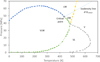 |
Fig. 14 Phase envelope obtained using Carnot for reservoir fluid evaluation using the critical density as reference for phase identification. V: vapor, L: organic liquid, W: aqueous phase. |
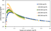 |
Fig. 15 Critical density surface calculated by the Heidemann–Khalil method using Carnot as a function of reservoir fluid composition. |
7 Carnot for research
Carnot is also used by IFPEN research staff (Ph.D. and post-doc researchers as well as interns) to allow new developments in the thermodynamic modeling of complex systems. To that end, a specific interface was designed so that computations can be performed using a formatted input file. The code then generates an output file that contains both the requested results and statistical values comparing the calculated values with the experimental ones. The flexibility of the C++ architecture is such that temporary research staff can easily contribute by developing specialized pieces of code, without worrying about the global complexity of phase equilibrium or other calculations. An example is provided in Figure 16, which shows the implementation of a generic equation of state. It is based on the formulation by Michelsen and Mollerup [108], who suggest expressing the equation of state using the residual Helmholtz energy Ares. All the residual properties are then computed straightforwardly using the derivatives with respect to the independent variables which are a number of moles, total volume, and temperature.
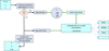 |
Fig. 16 Example of implementation of an equation of state (EoS). |
In Figure 16, it is visible that all Helmholtz energy contributions (such as dispersive, repulsive, associative, …) are handled separately, which makes it possible to adapt one piece without affecting the others. The resolution of the equation of state is a piece of code that is common to all such equations, and it also contains the possibility to check the quality of the analytical derivatives using numerical approximations.
7.1 Model parameterization
One of the first challenges when developing new models is the parameterization. It implies minimizing an objective function with respect to a set of parameters. To do such a parameter regression, an IFPEN platform named ATOUT (Advanced Tools for Optimization and Uncertainty Treatment) is used, which contains several functionalities like SQPAL [109], that allow minimization and statistical treatment of various functions. A Carnot R&D interface has been developed to generate files that can be read by ATOUT in the correct format. The objective function is then constructed within ATOUT as follows: where ns is the number of data series, nsj is the number of point values for data series j,
  is the weight multiplying coefficient for data series j, wji is the local weight for point i of data series j,
  is simulated data and
  are the experimental data.
Any type of property (series) can be included in the regression. The impact of each of the sub-functions on the global function can be evaluated, along with some important statistical values. Figure 17 shows an example of a parameter regression using ATOUT.
 |
Fig. 17 Illustration of the computation results from an ATOUT screenshot. The highlighted line is the best solution within the initial 50 points. |
Figure 17 shows, for each simulation (first column) the actual values of the parameters (columns “Alfa” till “TmsT”). These parameters are selected within the boundaries that are recalled in the bottom lines (Min and Max). Values for each of the sub-functions for the corresponding parameters are then listed, and the sum is provided in the last column. This way, it is made visible which of the properties (sub-functions) contributes most to the obtained minimum, and the weight factors can be adapted such that the desired balance is achieved.
Once an optimum solution is found, the tool allows for plotting response surfaces, thus making visible the sensitivity of any given parameter to either the global function or to any sub-function. An example of these response surfaces is provided in Figure 18.
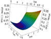 |
Fig. 18 Example of a response surface provided by the ATOUT framework. |
7.2 The GC-PPC-SAFT equation of state
Introduced by Chapman et al. three decades ago [110], the SAFT (Statistical Associating Fluid Theory) equation of state exhibits an increasing interest by researchers all over the world since it offers a significant improvement compared to usual equations of state like cubic equations. Thanks to a strong physical background, this model allows dealing with a large variety of systems, including apolar, polar, and associative molecules, electrolytes, polymers, etc. Using the framework of Carnot, Tamouza et al. [111, 112] was the first to develop a Group Contribution (GC) approach for the parameterization of the SAFT equation of state. The work was further pursued by Nguyen-Huynh et al. [113] who showed that using a polar term it was possible to significantly improve the predictive character of the model. A very good example is shown in Figure 19 showing the effect of benzene polarity on the isothermal phase diagram of the mixture with n-hexane. Further work along these lines was to include a predictive method for the kij parameter in the dispersive energy mixing rule [114, 115]. This SAFT version, named GC-PPC-SAFT (for Group Contribution Polar Perturbed Chain SAFT), is one of the most advanced versions of SAFT currently implemented in Carnot.
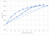 |
Fig. 19 Isothermal phase envelope of the n-hexane + benzene mixture at 298.15 K, with a comparison of experiments [116] and the non-polar PC-SAFT (dashed lines) and the polar PC-SAFT (solid line) as implemented in Carnot. |
Moreover, a specific type of mixing rule was found needed for hydrogen solubility computations in oxygenated compounds. This mixing rule, called “Non-Additive Hard Sphere” (NAHS) was developed [117] and introduced in the PC-SAFT framework [118] of Carnot. The predictive results are illustrated in Figure 20.
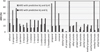 |
Fig. 20 Relative deviations of Henry’s constant of hydrogen in oxygenated solvents. Reproduced from [118]. |
It is worth mentioning that all specificities of the group contribution are introduced in the Carnot code, but that it can equally well use parameters from the literature using molecular parameters. The full group-contribution database is now available in the supplementary information of a recent publication that also compares the results with another parameterization method [119]. The code has been also implemented in the Simulis Thermodynamics package [8].
7.3 Electrolyte thermodynamics
Recently, a new research chair was started at IFPEN, focusing on electrolyte thermodynamics. Work has been performed with many different electrolyte models, including Pitzer, eUNIQUAC, and eNRTL [120]. Yet, a renewed effort has been made recently to work on electrolyte equations of state. The work was started in 2008 [121] by adding a long-range simplified MSA contribution to the CPA equation of state, along with a Born term. The e-CPA equation was further extended and applied to a specific context [122], requiring gas solubility modeling in high-temperature water.
Since 2013, the same long-range electrolyte terms have been added to the PC-SAFT equation of state [123]. The e-PPC-SAFT that is thus constructed may be parameterized in many different ways. A first parameterization study was performed by Roa-Pinto et al. [124] on a large database containing various types of data.
8 Conclusion
For more than twenty years, IFP Energies Nouvelles has been developing the thermodynamic library Carnot. Today, it contains around 20 equations of state: cubic EoS (PR, SRK) with a large variety of alpha functions and mixing rules, modern associative EoS such as CPA or SAFT, predictive EoS like GC-SAFT or PSRK, and several specific EoS. It also contains a dozen of activity coefficient models, from usual correlative models (NRTL, UNIQUAC, …) to predictive models such as UNIFAC and LIFAC. Electrolyte versions of both EoS and activity coefficient models are also implemented to deal with complex electrolyte systems: e-SAFT, Soreide & Whitson, e-UNIQUAC, Pitzer, etc. Furthermore, many specific models have been coded to compute various fluid properties, such as viscosities, interfacial properties, phase envelope, Henry’s constant, characterization of ill-defined mixtures, phase identification, etc. Carnot also contains a dozen flash algorithms making possible the computation of various types of phase equilibria, including not only fluid phase diphasic (VLE) and triphasic (VLLE) equilibria, but also configurations with solid phases such as hydrates, wax, asphaltene, or salts. Reactive flash algorithms have been also coded to couple phase equilibrium with chemical reaction processes, including either a stoichiometric (solving the law of mass action for a given set of reactions) or a non-stoichiometric (Gibbs free energy minimization) approach. Several specific algorithms are also present in Carnot, among them breakdown and distillation curve calculations, depletion simulations (constant mass expansion, constant volume depletion, differential liberation), fluid transportation facilities computations (valve, compressors, pump, heater), etc.
The informatics framework of Carnot, coded in C++, is extremely modular and allows for easily implementing new models and algorithms for both research and industry. It is worth noticing that an advanced system of versioning and non-regression tests makes Carnot compliant with the quality standards of the commercial software in which it is embedded.
Through some examples, this article demonstrated the wide range of usage that Carnot offers to industrial and R&D projects, in a large variety of energy-related areas: CO2 capture and storage, fluid transportation and flow assurance, chemistry, and geoscience. Consequently, Carnot is now the official thermodynamic kernel embedded in various commercial simulators, such as the PVT software Carbone™ [53] for reservoir simulation, the software TemisFlow™ [125] and CorresFlow™ [30] for basin modeling and CO2 storage, respectively, the software Moldi™ [38] for fluid transportation in pipes and risers, and the software Converge™ [126] for CFD modeling in combustion engines. Through these tools, several hundreds of end-users are nowadays performing their thermodynamic calculations with Carnot. It has also been used to design and optimize industrial processes such as the DMX™ process for CO2 capture, the ATOL® and BioButterFly™ solutions for bio-olefins production, and Futurol™ and BioTFuel™ for biofuels production. Finally, Carnot is also a powerful platform for R&D studies to develop and parameterize advanced thermodynamic models and algorithms for near-future applications.
The next developments in Carnot will concern not only the addition of new physical models but also a gradual incorporation of Artificial Intelligence (AI), including for instance the implementation of hybrid and neural-network approaches in complement to full-physical models. Some preliminary work has already shown interest in such an approach, as well as the gain expected by optimizing the informatic architecture of the code (GPU, vectorization, …) [67]. A strong complementarity between thermodynamics, machine learning, and computer science will be the key to enlarging the application range of Carnot in the future.
References
- United Nations. The 17 goals – sustainable development (un.org). Available at: https://sdgs.un.org/goals. [Google Scholar]
- de Hemptinne J.-C., Kontogeorgis G.M., Dohrn R., Economou I.G., Ten Kate A., Kuitunen S., Fele Žilnik L., de Angelis M.G., Vesovic V. (2022) A view on the future of applied thermodynamics, Ind. Eng. Chem. Res. 61, 39, 14664–14680. https://doi.org/10.1021/acs.iecr.2c01906. [CrossRef] [Google Scholar]
- van der Waals J.D. (1873) Over de continuiteit van den gas en vloeistoftestand (On the continuity of the gas and liquid state), Hoogeschool te Leiden. [Google Scholar]
- Calsep – PVTSim Nova. https://www.calsep.com/pvtsim-nova/. [Google Scholar]
- Petroleum Experts – PVTP. https://www.petex.com/products/ipm-suite/pvtp/. [Google Scholar]
- KBC – Multiflash. https://www.kbc.global/software/advanced-thermodynamics/. [Google Scholar]
- SPECS. https://www.cere.dtu.dk/expertise/software/specs. [Google Scholar]
- ProSim – Simulis Thermodynamics. https://www.prosim.net/en/product/simulis-thermodynamics-mixture-properties-and-fluid-phase-equilibria-calculations/. [Google Scholar]
- Bell I.H., Wronski J., Quoilin S., Lemort V. (2014) Pure and pseudo-pure fluid thermophysical property evaluation and the open-source thermophysical property library CoolProp, Ind. Eng. Chem. Res. 53, 6, 2498–2508. https://doi.org/10.1021/ie4033999. [CrossRef] [Google Scholar]
- Bell C.a.C. (2016–2020) Thermo: chemical properties component of chemical engineering design. https://github.com/CalebBell/thermo. [Google Scholar]
- Chaparro G., Mejía A. (2020) Phasepy: a Python based framework for fluid phase equilibria and interfacial properties computation, J. Comput. Chem. 41, 29, 2504–2526. https://doi.org/10.1002/jcc.26405. [CrossRef] [PubMed] [Google Scholar]
- Wilhelmsen Ø., Aasen A., Skaugen G., Aursand P., Austegard A., Aursand E., Gjennestad M.A., Lund H., Linga G., Hammer M. (2017) Thermodynamic modeling with equations of state: present challenges with established methods, Ind. Eng. Chem. Res. 56, 13, 3503–3515. https://doi.org/10.1021/acs.iecr.7b00317. [CrossRef] [Google Scholar]
- Rehner P., Bauer G. (2022) FeOs – a framework for equations of state and classical density functional theory. https://github.com/feos-org/feos. [Google Scholar]
- Bell I.H., Deiters U.K., Leal A.M.M. (2022) Implementing an equation of state without derivatives: teqp, Ind. Eng. Chem. Res. 61, 17, 6010–6027. https://doi.org/10.1021/acs.iecr.2c00237. [CrossRef] [Google Scholar]
- Walker P.J., Yew H.-W., Riedemann A. (2022) Clapeyron.jl: an extensible, open-source fluid thermodynamics toolkit, Ind. Eng. Chem. Res. 61, 20, 7130–7153. https://doi.org/10.1021/acs.iecr.2c00326. [CrossRef] [Google Scholar]
- https://www.swig.org/. [Google Scholar]
- https://www.colan.org/. [Google Scholar]
- Bai C., Dallasega P., Orzes G., Sarkis J. (2020) Industry 4.0 technologies assessment: a sustainability perspective, Int. J. Prod. Econ. 229, 107776. https://doi.org/10.1016/j.ijpe.2020.107776. [CrossRef] [Google Scholar]
- https://cmake.org/. [Google Scholar]
- http://google.github.io/googletest/. [Google Scholar]
- https://www.jenkins.io/. [Google Scholar]
- https://subversion.apache.org/. [Google Scholar]
- https://git-scm.com/. [Google Scholar]
- IEA (2022) Carbon capture, utilisation and storage, IEA, Paris. https://www.iea.org/reports/carbon-capture-utilisation-and-storage-2. [Google Scholar]
- https://www.ifpenergiesnouvelles.com/article/launch-innovative-european-3d-project-capture-and-storage-co2-industrial-scale. [Google Scholar]
- Tsanas C., Stenby E.H., Yan W. (2019) Calculation of multiphase chemical equilibrium in electrolyte solutions with non-stoichiometric methods, Fluid Phase Equilib. 482, 81–98. https://doi.org/10.1016/j.fluid.2018.10.008. [CrossRef] [Google Scholar]
- Deshmukh R.D., Mather A.E. (1981) A mathematical model for equilibrium solubility of hydrogen sulfide and carbon dioxide in aqueous alkanolamine solutions, Chem. Eng. Sci. 36, 2, 355–362. https://doi.org/10.1016/0009-2509(81)85015-4. [CrossRef] [Google Scholar]
- Chen C.C., Britt H.I., Boston J.F., Evans L.B. (1982) Local composition model for excess Gibbs energy of electrolyte systems. Part I: single solvent, single completely dissociated electrolyte systems, AIChE J. 28, 4, 588–596. [CrossRef] [Google Scholar]
- Tsanas C., de Hemptinne J.-C., Mougin P. (2022) Calculation of phase and chemical equilibrium for multiple ion-containing phases including stability analysis, Chem. Eng. Sci. 248, 117147. https://doi.org/10.1016/j.ces.2021.117174. [CrossRef] [Google Scholar]
- CooresFlow, https://www.ifpenergiesnouvelles.com/innovation-and-industry/our-expertise/climate-environment-and-circular-economy/co2-capture-storage-and-use/our-solutions. [Google Scholar]
- Estublier A., Fornel A., Brosse É., Houel P., Lecomte J.-C., Delmas J., Vincké O. (2017) Simulation of a potential CO2 storage in the West Paris Basin: site characterization and assessment of the long-term hydrodynamical and geochemical impacts induced by the CO2 Injection, Oil Gas Sci. Technol. Rev. IFP Energies nouvelles 72, 4. https://doi.org/10.2516/ogst/2017021. [Google Scholar]
- Soreide I., Whitson C. (1992) Peng-Robinson predictions for hydrocarbons, CO2, N2, and H2S with pure water and NaCl brine, Fluid Phase Equilib. 77, 217–240. [CrossRef] [Google Scholar]
- Chabab S., Théveneau P., Corvisier J., Coquelet C., Paricaud P., Houriez C., Ahmar E.E. (2019) Thermodynamic study of the CO2–H2O–NaCl system: Measurements of CO2 solubility and modeling of phase equilibria using Soreide and Whitson, electrolyte CPA and SIT models, Int. J. Greenhouse Gas Control 91, 102825. https://doi.org/10.1016/j.ijggc.2019.102825. [CrossRef] [Google Scholar]
- Yan W., Huang S., Stenby E.H. (2011) Measurement and modeling of CO2 solubility in NaCl brine and CO2–saturated NaCl brine density, Int. J. Greenhouse Gas Control 5, 6, 1460–1477. https://doi.org/10.1016/j.ijggc.2011.08.004. [CrossRef] [Google Scholar]
- Messabeb H., Contamine F., Cézac P., Serin J.P., Gaucher E.C. (2016) Experimental measurement of CO2 solubility in aqueous NaCl solution at temperature from 323.15 to 423.15 K and pressure of up to 20 MPa, J. Chem. Eng. Data 61, 10, 3573–3584. https://doi.org/10.1021/acs.jced.6b00505. [CrossRef] [Google Scholar]
- Koschel D., Coxam J.Y., Rodier L., Majer V. (2006) Enthalpy and solubility data of CO2 in water and NaCl (aq) at conditions of interest for geological sequestration, Fluid Phase Equilib. 247, 1–2, 107–120. [CrossRef] [Google Scholar]
- TechnipFMC, What we do. Available at: https://www.technipfmc.com/en/what-we-do/subsea/subsea-systems/subsea-infrastructure/flexible-pipes/. [Google Scholar]
- Aubry J.C., Saas J.N., Taravel-Condat C., Benjelloun-Dabaghi Z., de Hemptinne J.C. (2002) Moldi(Tm): a fluid permeation model to calculate the annulus composition in flexible pipes, Oil & Gas Sci. Technol. Rev. IFP 57, 2, 177–192. https://doi.org/10.2516/ogst:2002014. [CrossRef] [Google Scholar]
- Lefebvre X., Khvoenkova N., de Hemptinne J.-C., Lefrançois L., Radenac B., Pignoc-Chicheportiche S., Plennevaux C. (2022) Prediction of flexible pipe annulus composition by numerical modeling: identification of key parameters, Sci. Tech. Energy Transit. 77. https://doi.org/10.2516/stet/2022008. [Google Scholar]
- Kontogeorgis G.M., Voutsas E.C., Yakoumis I.V., Tassios D.P. (1996) An equation of state for associating fluids, Ind. Eng. Chem. Res. 35, 11, 4310–4318. [CrossRef] [Google Scholar]
- Gross J., Sadowski G. (2001) Perturbed-chain SAFT: an equation of state based on a perturbation theory for chain molecules, Ind. Eng. Chem. Res. 40, 1244–1260. [CrossRef] [Google Scholar]
- de Boer R.B., Leerlooyer K., Eigner M.R.P., van Bergen A.R.D. (1995) Screening of crude oils for asphalt precipitation: theory, practice, and the selection of inhibitors, SPE Prod. Facil. 10, 1, 55–61. https://doi.org/10.2118/24987-PA. [CrossRef] [Google Scholar]
- Buenrostro-Gonzalez E., Lira-Galeana C., Gil-Villegas A., Wu J. (2004) Asphaltene precipitation in crude oils: theory and experiments, AIChE J. 50, 10, 2552–2570. https://doi.org/10.1002/aic.10243. [CrossRef] [Google Scholar]
- Szewczyk V. (1997) Modélisation thermodynamique compositionelle de la floculation des bruts asphalténiques, PhD Thesis, INPL, Vandoeuvre-les-Nancy, France. [Google Scholar]
- Szewczyk V., Behar E. (1999) Compositional model for predicting asphaltene flocculation, Fluid Phase Equilib. 158–160, 459–469. [CrossRef] [Google Scholar]
- Mougin P., Behar E., Szewczyk V. Floculation des bruts asphalténiques: Présentation d’un modèle compositionnel, IFPEN Internal Report 44460, 1998. [Google Scholar]
- Pina A., Mougin P. Modélisation des seuils de floculation par ajout de solvant/floculant. Incidence du choix du module de calcul de flash, IFPEN Internal Report 53130, 2000. [Google Scholar]
- Peneloux A., Abdoul W., Rauzy E. (1989) Excess functions and equations of state, Fluid Phase Equilib. 47, 2–3, 115–132. [CrossRef] [Google Scholar]
- Abdoul W., Rauzy E., Peneloux A. (1991) Group-contribution equation of state for correlating and predicting thermodynamic properties of weakly polar and non-associating mixtures; binary and multicomponent systems, Fluid Phase Equilib. 68, 47–102. [CrossRef] [Google Scholar]
- Jaubert J.N., Mutelet F. (2004) VLE predictions with the Peng–Robinson equation of state and temperature dependent kij calculated through a group contribution method, Fluid Phase Equilib. 224, 285–304. [CrossRef] [Google Scholar]
- Qian J.-W., Privat R., Jaubert J.-N. (2013) Predicting the phase equilibria, critical phenomena, and mixing enthalpies of binary aqueous systems containing alkanes, cycloalkanes, aromatics, alkenes, and gases (N2, CO2, H2S, H2) with the PPR78 equation of state, Ind. Eng. Chem. Res. 52, 46, 16457–16490. [CrossRef] [Google Scholar]
- Li Z., Firoozabadi A. (2010) Cubic-plus-association equation of state for asphaltene precipitation in live oils, Energy Fuel 24, 5, 2956–2963. https://doi.org/10.1021/ef9014263. [CrossRef] [Google Scholar]
- Carbone - Kappa Engineering. https://www.kappaeng.com/software/carbone. [Google Scholar]
- Eslamimanesh A., Mohammadi A.H., Richon D., Naidoo P., Ramjugernath D. (2012) Application of gas hydrate formation in separation processes: a review of experimental studies, J. Chem. Thermodyn. 46, 62–71. https://doi.org/10.1016/j.jct.2011.10.006. [CrossRef] [Google Scholar]
- Van der Waals J.H., Platteeuw J.C. (1959) Clathrate solutions, Adv. Chem. Phys. 2, 1, 1–57. [Google Scholar]
- Deaton W.M., Frost E.M. Jr. (1946) Gas hydrates and their relation to the operation of natural-gas pipe lines, vol. 8, U.S. Bureau of Mines Monograph, 101p. [Google Scholar]
- Kobayashi R., Katz D.L. (1949) Methane Hydrate at High Pressure, J. Petrol. Technol. 1, 3, 66–70. https://doi.org/10.2118/949066-G. [CrossRef] [Google Scholar]
- Makogon T.Y., Sloan E.D. Jr. (1994) Phase equilibrium for methane hydrate from 190 to 262 K, J. Chem. Eng. Data 39, 2, 351–353. https://doi.org/10.1021/je00014a035. [CrossRef] [Google Scholar]
- Falabella B.J. (1975) A study of natural gas hydrates, University of Massachusetts. [Google Scholar]
- van Cleeff A., Diepen G.A.M. (1960) Gas hydrates of nitrogen and oxygen, Recl. Trav. Chim. Pays-Bas 79, 6, 582–586. https://doi.org/10.1002/recl.19600790606. [Google Scholar]
- Vinš V., Jäger A., Hrubý J., Span R. (2017) Model for gas hydrates applied to CCS systems part II. Fitting of parameters for models of hydrates of pure gases, Fluid Phase Equilib. 435, 104–117. https://doi.org/10.1016/j.fluid.2016.12.010. [CrossRef] [Google Scholar]
- Circone S., Stern L.A., Kirby S.H., Durham W.B., Chakoumakos B.C., Rawn C.J., Rondinone A.J., Ishii Y. (2003) CO2 hydrate: synthesis, composition, structure, dissociation behavior, and a comparison to structure I CH4 hydrate, J. Phys. Chem. B 107, 23, 5529–5539. https://doi.org/10.1021/jp027391j. [CrossRef] [Google Scholar]
- Hester K.C., Huo Z., Ballard A.L., Koh C.A., Miller K.T., Sloan E.D. (2007) Thermal expansivity for sI and sII clathrate hydrates, J. Phys. Chem. B 111, 30, 8830–8835. https://doi.org.10.1021/jp0715880. [CrossRef] [PubMed] [Google Scholar]
- Ikeda T., Mae S., Yamamuro O., Matsuo T., Ikeda S., Ibberson R.M. (2000) Distortion of host lattice in clathrate hydrate as a function of guest molecule and temperature, J. Phys. Chem. A 104, 46, 10623–10630. https://doi.org/10.1021/jp001313j. [CrossRef] [Google Scholar]
- Yang S., Ping Y., Habchi C. (2019) Real-fluid injection modeling and LES simulation of the ECN spray a injector using a fully compressible two-phase flow approach, Int. J. Multiphase Flow 122. https://doi.org/10.1016/j.ijmultiphaseflow.2019.103145. [Google Scholar]
- Gaballa H., Jafari S., Habchi C., de Hemptinne J.-C. (2022) Numerical investigation of droplet evaporation in high-pressure dual-fuel conditions using a tabulated real-fluid model, Int. J. Heat Mass Transfer 189. https://doi.org/10.1016/j.ijheatmasstransfer.2022.122671. [CrossRef] [Google Scholar]
- Qu J., Faney T., de Hemptinne J.-C., Yousef S., Gallinari P. (2023) PTFlash: a vectorized and parallel deep learning framework for two-phase flash calculation, Fuel 331, 125603. https://doi.org/10.1016/j.fuel.2022.125603. [CrossRef] [Google Scholar]
- Itani L.M., Bruneaux G., Di Lella A., Schulz C. (2015) Two-tracer LIF imaging of preferential evaporation of multi-component gasoline fuel sprays under engine conditions, Proc. Combust. Inst. 35, 3, 2915–2922. https://doi.org/10.1016/j.proci.2014.06.108. [CrossRef] [Google Scholar]
- Holderbaum T.G. (1991) PSRK: a group contribution equation of state based on UNIFAC, Fluid Phase Equilib. 70, 251–265. [CrossRef] [Google Scholar]
- https://www.axens.net/markets/renewable-fuels-bio-based-chemicals/bio-olefins. [Google Scholar]
- https://www.axens.net/markets/renewable-fuels-bio-based-chemicals/renewable-diesel-and-jet. [Google Scholar]
- Twu C.H., Bluck D., Cunningham J.R., Coon J.E. (1991) A cubic equation of state with a new alpha function and a new mixing rule, Fluid Phase Equilib. 69, 33–50. [CrossRef] [Google Scholar]
- Mackay E.J. (2003) Modeling in-situ scale deposition: the impact of reservoir and well geometries and kinetic reaction rates, SPE Prod. Facil. 18, 1, 45–56. https://doi.org/10.2118/81830-PA. [CrossRef] [Google Scholar]
- Moghadasi J., Jamialahmadi M., Müller-Steinhagen H., Sharif A., Ghalambor A., Izadpanah M.R., Motaie E. (2003) Scale formation in Iranian oil reservoir and production equipment during water injection, OnePetro. [Google Scholar]
- Bin Merdhah A.B., Yassin A.M. (2007) Study of scale formation in oil reservoir during water injection-a review. Available at: https://www.researchgate.net/publication/277791130_Study_of_scale_formation_in_oil_reservoir_during_water_injection-A_review . [Google Scholar]
- Pitzer K.S. (1973) Thermodynamics of electrolytes I: theoretical basis and general equations, J. Phys. Chem. 77, 2, 268–277. [CrossRef] [Google Scholar]
- Pitzer K.S. (1975) Thermodynamics of electrolytes. V. Effects of high order electrostatic terms, J. Sol. Chem. 4, 249–265. [CrossRef] [Google Scholar]
- Pitzer K.S., Peiper J.C., Busey R.H. (1984) Thermodynamic properties of aqueous sodium chloride solutions, J. Phys. Chem. Ref. Data 13, 1, 1–102. [CrossRef] [Google Scholar]
- Haaberg T., Jakobsen J.E., Østvold T. (1990) The effect of Ferrous iron on mineral scaling during oil recovery, Acta Chem. Scand. 44, 907–915. [CrossRef] [Google Scholar]
- Pedersen K.S., Christensen P.L., Shaikh J.A., Christensen P.L. (2006) Phase Behavior of Petroleum Reservoir Fluids, CRC Press. ISBN 9780429120855. [CrossRef] [Google Scholar]
- Anderson G.M., Burnham C.W. (1965) The solubility of quartz in super-critical water, Am. J. Sci. 263, 6, 494. https://doi.org/10.2475/ajs.263.6.494. [CrossRef] [Google Scholar]
- Crerar D.A., Anderson G.M. (1971) Solubility and solvation reactions of quartz in dilute hydrothermal solutions, Chem. Geol. 8, 2, 107–122. https://doi.org/10.1016/0009-2541(71)90052-0. [CrossRef] [Google Scholar]
- Kennedy G.C. (1950) A portion of the system silica-water, Econ. Geol. 45, 7, 629–653. https://doi.org/10.2113/gsecongeo.45.7.629. [CrossRef] [Google Scholar]
- Khitarov N.I. (1956) The 400 °C isotherm for the system H2O–SiO2 at pressures up to 2,000 kg/cm2, Geochem. Int. 1956, 55–61. [Google Scholar]
- Kitahara S. (1960) The solubility of quartz in water at high temperature and high pressures, Rev. Phys. Chem. Japan 30, 109–114. [Google Scholar]
- Manning C.E. (1994) The solubility of quartz in H2O in the lower crust and upper mantle, Geochim. Cosmochim. Acta 58, 22, 4831–4839. https://doi.org/10.1016/0016-7037(94)90214-3. [CrossRef] [Google Scholar]
- Morey George W., Fournier Robert Orville, Rowe J.J. (1964) The solubility of amorphous silica at 25 C, J. Geophys. Res. 69, 1995–2002. [CrossRef] [Google Scholar]
- Morey G., Fournier R., Rowe J. (1962) The solubility of quartz in water in the temperature interval from 25 to 300 C, Geochim. Cosmochim. Acta 26, 10, 1029–1043. https://doi.org/10.1016/0016-7037(62)90027-3. [CrossRef] [Google Scholar]
- Vala Ragnarsdóttir K., Walther J.V. (1983) Pressure sensitive “silica geothermometer” determined from quartz solubility experiments at 250 °C, Geochim. Cosmochim. Acta 47, 5, 941–946. https://doi.org/10.1016/0016-7037(83)90159-X. [CrossRef] [Google Scholar]
- Rimstidt J. (1997) Quartz solubility at low temperatures, Geochim. Cosmochim. Acta 61, 13, 2553–2558. https://doi.org/10.1016/S0016-7037(97)00103-8. [CrossRef] [Google Scholar]
- Sue K., Mizutani T., Usami T., Arai K., Kasai H., Nakanishi H. (2004) Titanyl phthalocyanine solubility in supercritical acetone, J. Supercrit. Fluids 30, 3, 281–285. https://doi.org/10.1016/j.supflu.2003.09.008. [CrossRef] [Google Scholar]
- Wang H.M., Henderson G.S., Brenan J.M. (2004) Measuring quartz solubility by in situ weight-loss determination using a hydrothermal diamond cell, Geochim. Cosmochim. Acta 68, 24, 5197–5204. https://doi.org/10.1016/j.gca.2004.06.006. [CrossRef] [Google Scholar]
- Weill D., Fyfe W. (1964) The solubility of quartz in H2O in the range 1000–4000 bars and 400–550 °C, Geochim. Cosmochim. Acta 28, 8, 1243–1255. https://doi.org/10.1016/0016-7037(64)90126-7. [CrossRef] [Google Scholar]
- Yokoyama C., Iwabuchi A., Takahashi S., Takeuchi K. (1993) Solubility of PbO in supercritical water, Fluid Phase Equilib. 82, 323–331. https://doi.org/10.1016/0378-3812(93)87156-U. [CrossRef] [Google Scholar]
- Ozarslan A. (2012) Large-scale hydrogen energy storage in salt caverns, Int. J. Hydrogen Energy 37, 19, 14265–14277. https://doi.org/10.1016/j.ijhydene.2012.07.111. [CrossRef] [Google Scholar]
- Réveillère A., Londe L. (2017) Compressed air energy storage: a new beginning? geostock, France, in: SMRI Fall Meeting, Münster, Germany. [Google Scholar]
- Roa Pinto J.S., Bachaud P., Fargetton T., Ferrando N., Jeannin L., Louvet F. (2021) Modeling phase equilibrium of hydrogen and natural gas in brines: application to storage in salt caverns, Int. J. Hydrogen Energy 46, 5, 4229–4240. https://doi.org/10.1016/j.ijhydene.2020.10.242. [CrossRef] [Google Scholar]
- Kiemde A.F., Ferrando N., de Hemptinne J.C., Le Gallo Y., Reveillere A., Roa Pinto J.S. (2003) Hydrogen and Air Storage in Salt Caverns: a thermodynamic model for phase equilibrium calculations, Sci. Technol. Energy Transit. Energy 78, 10. [Google Scholar]
- Chabab S., Théveneau P., Coquelet C., Corvisier J., Paricaud P. (2000) Measurements and predictive models of high-pressure H2 solubility in brine (H2O+NaCl) for underground hydrogen storage application, Int. J. Hydrogen Energy 45, 32206–32200. https://doi.org/10.1016/j.ijhydene.2020.08.192. [CrossRef] [Google Scholar]
- Schneider F., Wolf S., Faille I., Pot D. (2000) A 3d basin model for hydrocarbon potential evaluation: application to congo offshore, Oil Gas Sci. Technol. Rev. IFP 55, 1, 3–13. https://doi.org/10.2516/ogst:2000001. [CrossRef] [Google Scholar]
- Willien F., Chetvchenko I., Masson R., Quandalle P., Agelas L., Requena S. (2009) AMG preconditioning for sedimentary basin simulations in Temis calculator, Mar. Pet. Geol. 26, 4, 519–524. https://doi.org/10.1016/j.marpetgeo.2009.01.014. [CrossRef] [Google Scholar]
- Thibaut M., Jardin A., Faille I., Willien F., Guichet X. (2014) Advanced workflows for fluid transfer in faulted basins, Oil Gas Sci. Technol. Rev. IFP Energies Nouvelles 69, 4, 573–584. https://doi.org/10.2516/ogst/2014016. [CrossRef] [Google Scholar]
- Ungerer P., Burrus J., Doligez B.P.Y.C., Chenet P.Y., Bessis F. (1990) Basin evaluation by integrated two-dimensional modeling of heat transfer, fluid flow, hydrocarbon generation, and migration, AAPG Bull. 74, 3, 309–335. https://doi.org/10.1306/0C9B22DB-1710-11D7-8645000102C1865D [Google Scholar]
- Meiller C., Coatléven J., Maurand N., Guichet X. (2017) Ecoulements triphasiques dans les bassins sédimentaires, Géologues 193, 54–58. [Google Scholar]
- Jayanti P.C., Venkatarathnam G. (2016) Identification of the phase of a substance from the derivatives of pressure, volume and temperature, without prior knowledge of saturation properties: Extension to solid phase, Fluid Phase Equilib. 425, 269–277. https://doi.org/10.1016/j.fluid.2016.06.001. [CrossRef] [Google Scholar]
- Venkatarathnam G., Oellrich L.R. (2011) Identification of the phase of a fluid using partial derivatives of pressure, volume, and temperature without reference to saturation properties: applications in phase equilibria calculations, Fluid Phase Equilib. 301, 2, 225–233. https://doi.org/10.1016/j.fluid.2010.12.001. [CrossRef] [Google Scholar]
- Heidemann R.A., Khalil A.M. (1980) The calculation of critical points, AIChE J. 26, 5, 769–779. https://doi.org/10.1002/aic.690260510. [CrossRef] [MathSciNet] [Google Scholar]
- Michelsen M.L., Mollerup J. (2004) Thermodynamic models: fundamental and computational aspects, Tie-Line Publications. ISBN: 87-989961-1-8 [Google Scholar]
- Delbos F., Gilbert J.C., Sinoquet D. (2003) Application of an SQP augmented Lagrangian method to a large-scale problem in 3D reflection tomography, in: ISMP 2003, 18th International Symposium on Mathematical Programming, Copenhagen, Aug. 18–22, p. 61. [Google Scholar]
- Chapman W.G., Gubbins K.E., Jackson G., Radosz M. (1989) SAFT: equation-of-state solution model for associating fluids, Fluid Phase Equilib. 52, 31–38. https://doi.org/10.1016/0378-3812(89)80308-5. [CrossRef] [Google Scholar]
- Tamouza S., Passarello J.P., Tobaly P., de Hemptinne J.C. (2004) Group contribution method with SAFT EOS applied to vapor liquid equilibria of various hydrocarbon series, Fluid Phase Equilib. 222–223, 67–76. [CrossRef] [Google Scholar]
- Tamouza S., Passarello J.P., Tobaly P., de Hemptinne J.C. (2005) Application to binary mixtures of a group contribution SAFT EOS, Fluid Phase Equilib. 228–229, 409–419. [CrossRef] [Google Scholar]
- Nguyen Huynh D., Passarello J.-P., Tobaly P., de Hemptinne J.-C. (2008) Application of GC-SAFT EOS to polar systems using a segment approach, Fluid Phase Equilib. 264, 1, 62–75. https://doi.org/10.1016/j.fluid.2007.10.019. [CrossRef] [Google Scholar]
- Nguyen-Huynh D., Passarello J.P., Tobaly P., de Hemptinne J.C. (2008) Modeling phase equilibria of asymmetric mixtures using a group-contribution SAFT (GC-SAFT) with a kij correlation method based on London’s theory. 1. Application to CO2 + n-alkane, methane + n-alkane, and ethane + n-alkane systems, Ind. Eng. Chem. Res. 47, 22, 8847–8858. [CrossRef] [Google Scholar]
- Nguyen-Huynh D., Tran T.K.S., Tamouza S., Passarello J.P., Tobaly P., de Hemptinne J.C. (2008) Modeling phase equilibria of asymmetric mixtures using a group-contribution SAFT (GC-SAFT) with a kij correlation method based on London’s theory. 2. Application to binary mixtures containing aromatic hydrocarbons, n-Alkanes, CO2, N2, and H2S, Ind. Eng. Chem. Res. 47, 22, 8859–8868. [CrossRef] [Google Scholar]
- Smith V.C., Robinson R.L., Jr. (1970) Vapor–liquid equilibriums at 25.deg. in the binary mixtures formed by hexane, benzene, and ethanol, J. Chem. Eng. Data 15, 3, 391–395. https://doi.org/10.1021/je60046a005. [CrossRef] [Google Scholar]
- Trinh T.-K.-H., Passarello J.-P., de Hemptinne J.-C., Lugo R., Lachet V. (2016) A non-additive repulsive contribution in an equation of state: The development for homonuclear square well chains equation of state validated against Monte Carlo simulation, J. Chem. Phys. 144, 12, 124902. https://doi.org/10.1063/1.4944068. [CrossRef] [PubMed] [Google Scholar]
- Trinh T.-K.-H., Passarello J.-P., de Hemptinne J.-C., Lugo R. (2016) Use of a non additive GC-PPC-SAFT equation of state to model hydrogen solubility in oxygenated organic compounds, Fluid Phase Equilib. 429, 177–195. https://doi.org/10.1016/j.fluid.2016.08.003. [CrossRef] [Google Scholar]
- Creton B., Agoudjil C., de Hemptinne J.-C. (2023) Assessment of two PC-SAFT parameterization strategies for pure compounds: model accuracy and sensitivity analysis, Fluid Phase Equilib. 565, 113666. https://doi.org/10.1016/j.fluid.2022.113666. [CrossRef] [Google Scholar]
- Yang F., Ngo T.D., Kontogeorgis G.M., de Hemptinne J.-C. (2022) A benchmark database for mixed-solvent electrolyte solutions: consistency analysis using E-NRTL, Ind. Eng. Chem. Res. 61, 42, 15576–15593. https://doi.org/10.1021/acs.iecr.2c00059. [CrossRef] [Google Scholar]
- Inchekel R., de Hemptinne J.C., Fürst W. (2008) The simultaneous representation of dielectric constant, volume and activity coefficients using an electrolyte equation of state, Fluid Phase Equilib. 271, 1–2, 19–27. [CrossRef] [Google Scholar]
- Courtial X., Ferrando N., de Hemptinne J.-C., Mougin P. (2014) Electrolyte CPA equation of state for very high temperature and pressure reservoir and basin applications, Geochim. Cosmochim. Acta 142, 1–14. https://doi.org/10.1016/j.gca.2014.07.028. [CrossRef] [Google Scholar]
- Rozmus J., de Hemptinne J.C., Galindo A., Dufal S., Mougin P. (2013) Modeling of strong electrolytes with ePPC-SAFT up to high temperatures, Ind. Eng. Chem. Res. 52, 9979–9994. https://doi.org/10.1021/ie303527j. [CrossRef] [Google Scholar]
- Roa Pinto J.S., Ferrando N., de Hemptinne J.-C., Galindo A. (2022) Temperature dependence and short-range electrolytic interactions within the e-PPC-SAFT framework, Fluid Phase Equilib. 560, 113486. https://doi.org/10.1016/j.fluid.2022.113486. [CrossRef] [Google Scholar]
- TemisFlow. https://www.beicip.com/petroleum-system-assessment. [Google Scholar]
- Converge. https://convergecfd.com/. [Google Scholar]
All Tables
All Figures
|
Fig. 1 Concentration profiles of a DMX solution with CO2. The DMX solvent is composed of water and two amines: DMX-A & DMX-B. Calculations done with the Deshmukh and Mather model in Carnot. |
| In the text | |
|
Fig. 2 Isotherms of CO2 capture by a DMX-A solution. Symbols are experimental data and lines are model results. Calculations done with the Deshmukh and Mather model in Carnot. |
| In the text | |
|
Fig. 3 CO2 solubility in pure water and in brines (NaCl) at 373.15 K. Symbols: experiments [33–36] (open squares: in pure water; triangles: salinity = 1 mol/kg; diamonds: salinity = 3 mol/kg; squares: salinity = 5 mol/kg; circles: salinity = 6 mol/kg). Lines: calculation with the S&W model in Carnot. |
| In the text | |
|
Fig. 4 The de Boer plot illustrating (Pr–Pb = difference between the reservoir pressure and the bubble pressure of the fluid) versus the fluid density. The red point corresponds to the fluid C1 from [43]. |
| In the text | |
|
Fig. 5 Bubble pressure and asphaltene precipitation upper onset pressure (UAOP) as function of the temperature for the reservoir fluid C1 [43] (a) and weight fraction of precipitated asphaltenes (b). |
| In the text | |
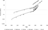 |
Fig. 6 Hydrate formation predictions with Carnot (lines). Experimental data (symbols) from [56–60]. |
| In the text | |
|
Fig. 7 CO2 hydrate lattice parameter calculated with Carnot and compared with experimental data [61–64]. |
| In the text | |
|
Fig. 8 Distillation curves and tracer profiles of a biofuel. From [68]. All simulations are performed with Carnot. |
| In the text | |
|
Fig. 9 Phase diagram of the binary mixture water + 1-butanol at atmospheric pressure. Symbols: experimental data. Lines: SRK-Twu model (Carnot). |
| In the text | |
|
Fig. 10 Saturation index of various salts versus temperature at pressure of 10 bar. The composition of the water is in Table 3. |
| In the text | |
|
Fig. 11 Simulated results of scale deposit when mixing formation and seawater at 25 °C and 1 bar: saturation index (a) and quantity of precipitated salts (b) versus volume fraction of seawater. |
| In the text | |
|
Fig. 12 Comparison between experimental data [81–94] and predicted silica solubilities in pure water from 20 °C to 900 °C and pressure up to 20,000 bar. |
| In the text | |
|
Fig. 13 Predictions of hydrogen solubility in salted water at 323 K (left) and 373 K (right). Lines: e-PPC-SAFT model. Symbols: experimental data not used in the parameterization database [99]. Orange diamonds: 1 mol/kg. Green triangles: 3 mol/kg. Blue circles: 5 mol/kg. |
| In the text | |
|
Fig. 14 Phase envelope obtained using Carnot for reservoir fluid evaluation using the critical density as reference for phase identification. V: vapor, L: organic liquid, W: aqueous phase. |
| In the text | |
|
Fig. 15 Critical density surface calculated by the Heidemann–Khalil method using Carnot as a function of reservoir fluid composition. |
| In the text | |
|
Fig. 16 Example of implementation of an equation of state (EoS). |
| In the text | |
|
Fig. 17 Illustration of the computation results from an ATOUT screenshot. The highlighted line is the best solution within the initial 50 points. |
| In the text | |
|
Fig. 18 Example of a response surface provided by the ATOUT framework. |
| In the text | |
|
Fig. 19 Isothermal phase envelope of the n-hexane + benzene mixture at 298.15 K, with a comparison of experiments [116] and the non-polar PC-SAFT (dashed lines) and the polar PC-SAFT (solid line) as implemented in Carnot. |
| In the text | |
|
Fig. 20 Relative deviations of Henry’s constant of hydrogen in oxygenated solvents. Reproduced from [118]. |
| In the text | |
Current usage metrics show cumulative count of Article Views (full-text article views including HTML views, PDF and ePub downloads, according to the available data) and Abstracts Views on Vision4Press platform.
Data correspond to usage on the plateform after 2015. The current usage metrics is available 48-96 hours after online publication and is updated daily on week days.
Initial download of the metrics may take a while.