")
")
| Issue |
Sci. Tech. Energ. Transition
Volume 81, 2026
Enabling Technologies for the Integration of Electrical Systems in Sustainable Energy Conversion
|
|
|---|---|---|
| Article Number | 3 | |
| Number of page(s) | 17 | |
| DOI | https://doi.org/10.2516/stet/2026010 | |
| Published online | 24 March 2026 | |
Regular Article
Advanced algorithm for fault detection and localization in DC microgrids utilizing capacitor current transient analysis for enhanced reliability in DER-integrated systems
Department of Electrical Engineering, Maulana Azad National Institute of Technology, Bhopal 462003, MP, India
* Corresponding author: This email address is being protected from spambots. You need JavaScript enabled to view it.
Received:
16
April
2025
Accepted:
10
February
2026
Abstract
This paper presents an advanced Short-Circuit (SC) fault detection and location methodology for DC Microgrids (DCMGs) integrating Distributed Energy Resources (DERs). Unisolated SC faults in DC systems present a significant challenge, leading to service disruptions and hindering effective fault detection. To address this, the proposed method capitalizes on the capacitor-dominated characteristics of DCMGs by utilizing capacitor current dynamics. A comprehensive DCMG system model is developed to facilitate the application and evaluation of the proposed scheme. The algorithm employs the average capacitor current and cable resistance to accurately determine the occurrence and location of faults within the DCMG network. Active DER sources (solar PV, wind, utility grid, and batteries) connect to loads via DC–DC converters, cables, relays, and circuit breakers. The method effectively detects the average capacitor current, enabling the identification of internal faults. Faults are classified as external if a set criterion is not met. Furthermore, the paper proposes a redundancy-based isolation configuration for zonal-type distributed networks. The efficacy of the methodology is rigorously validated through digital simulation studies. MATLAB/Simulink simulations of a DCMG, incorporating diverse generation sources and loads, are conducted under various fault scenarios. These include internal and external faults, as well as Line-to-Ground (LG) and Line-to-Line (LL) faults. The simulation results demonstrate the method’s ability to accurately detect both Low-Impedance Faults (LIFs) and High-Impedance Faults (HIFs) and to locate the faulty cable. Notably, the approach achieves fault cable detection and isolation within 2.3 ms, confirming its effectiveness and speed.
Key words: DC microgrid (DCMG) / Capacitor current / Fault detection / Fault location / Low-impedance fault (LIF) / High-impedance fault (HIF) / Relay
© The Author(s), published by EDP Sciences, 2026
 This is an Open Access article distributed under the terms of the Creative Commons Attribution License (https://creativecommons.org/licenses/by/4.0), which permits unrestricted use, distribution, and reproduction in any medium, provided the original work is properly cited.
1 Introduction
Achieving integration of Distributed Energy Resources (DER) such as solar PhotoVoltaic (PV) systems, wind turbines, battery storage, and utility grids into DC Microgrids (DCMGs) has always remained a challenge. Modern methods usually involve reducing DER and using contemporary power electronic converters [1] to improve integration. These converters enable the coupling of DC power components [2]. A DCMG, or grid system that integrates DERs and loads, offers significant advantages over AC systems, making DER integration more feasible [3, 4]. However, DCMG faces practical implementation issues, such as protection schemes, bidirectional power-flow management, stability maintenance and control, dealing with low inertia, and accurate system modelling [5, 6].
The DCMG network protection requires unique strategies and faces complex security obstacles. Unlike AC systems, DC fault currents exhibit distinct characteristics that complicate protection. Rapidly rising fault currents, driven by DC bus capacitor discharge during short circuits, present a significant challenge [7, 8]. DC faults don’t have zero crossings, which makes it more difficult for conventional breaker interruption. Therefore, specialized breakers and converter setups are often needed for effective fault clearing [9, 10]. Consequently, traditional AC protection methods are often unsuitable for DC systems [11–13]. The faults in microgrids can be broadly classified as AC-side faults, DC-side faults, and internal converter faults [14–16]. AC-side faults can arise from transmission or distribution line short circuits, AC-side converter failures, or conductor breaks [17]. The DC-side faults include short circuits like Line-to-Ground (LG) and Line-to-Line (LL) faults, as well as arc faults [18, 19]. The converter failures or malfunctions are categorized as internal converter faults [20]. Short-Circuit (SC) faults are particularly dangerous due to the low-resistance path they provide for high fault currents, necessitating rapid detection to prevent accidents [21, 22]. Various fault detection methods for DC systems have been proposed, utilizing techniques such as differential current, voltage sag analysis, and equivalent resistance calculation. Additionally, travelling wave analysis, Wavelet Transform (WT), and Artificial Neural Networks (ANNs) have also been employed [23, 24]. Although some methods provide faster identification speed, their practical implementation costs can be prohibitive [25, 26]. In addition to detection, accurate fault localization is crucial for restoring service after isolating the faulted section, minimizing power interruptions for end-users. Effective fault localization algorithms are thus necessary for rapid system recovery [27].
In [28, 29], several research articles have focused specifically on DCMG fault detection methods. In [30, 31], an iterative algorithm for fault detection in DCMG is presented. If there is a fault, the rate of the current rise in the DCMG is very high. It has a good ability to detect High-Impedance Faults (HIFs) and Low-Impedance Faults (LIFs), but it requires both voltage and current thresholds to detect these types of faults. However, overcurrent relays (RS) coordination is complicated due to the DCMG’s low resistance and short cable length. Several fast protection methods for DCMGs have been developed. In [32], one approach uses the magnitude of the current difference in line segments for rapid fault detection. In [33–35], other methods identify faults based on the sign of estimated line parameters. In [36], a transient-based fault detection method has also been proposed, though it cannot differentiate between internal and external faults. In [37, 38], a discrete frame differential current method for PV-based multiterminal DCMG has also been explored. In [39], recognizing the challenges of overcurrent-based fault detection in DCMG. In [40, 41], a non-unit protection scheme using overcurrent and current/voltage change rate has been proposed. In [42, 43], research has also specifically addressed DCMG fault location. One technique involves connecting an external circuit at both ends of the line for DC fault location, but its accuracy is affected by fault resistance. As demonstrated, recent research has largely focused on either fault detection or fault location within DCMGs, highlighting the need for comprehensive solutions. Recently, [44] explored high-frequency signal injection for DC protection, enhancing detection speed, while [45] addressed energy storage-related protection under renewable fluctuations. Meanwhile, [46, 47] reviewed fault localization in distributed networks using probabilistic approaches, complementing existing deterministic schemes.
In [48], a high-speed current differential method was implemented in a smart DC distribution system, utilizing DC differential current characteristics for fault detection. This unit-based approach requires a substantial number of RS (e.g., 10, as depicted in Fig. 1) for transmission line protection. In [49], resistance-based fault detection for localizing LIFs was proposed. In [50], a local resistance-based SC fault detection method for zonal DCMG was developed. However, a key limitation of the zonal approach is that a fault near a load can result in the isolation of all loads. Furthermore, the increased number of RS contributes to the system cost. In [51], combined fault detection and localization in DCMGs have been explored in a limited number of studies. In [52], one such approach uses a multi-criteria system for fault detection and a neural network for estimating fault distance. In [53], another method employs overcurrent protection for fault detection in DCMGs, using a probe power unit for fault location. In [54], a transient-based technique detects faults by comparing transient and steady-state currents, followed by fault location prediction via simulation analysis of sampled and estimated currents. However, the accuracy of both fault detection and localization in this method is susceptible to high-resistance faults. To address these challenges, [55] introduced an AI-based diagnostic tool leveraging energy conversion signatures, while [56] proposed a novel energy-aware adaptive protection system that reduces false tripping under variable DER conditions. These examples underscore the need for robust and cost-effective fault management strategies in DCMGs.
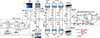 |
Fig. 1 Schematic diagram of a DC microgrid along with different types of DERs and loads. |
Short-time Fourier Transform (FT) and WT-based fault detection methods that rely on DC variations have been reported [57]. However, these methods are susceptible to high transmission resistance [58]. To address SC fault detection in capacitor-dominated grids, a novel scheme is proposed [59]. This article introduces a unit fault detection and localization algorithm for DCMG systems, aiming to overcome the limitations of existing techniques [60]. The algorithm estimates fault location online using voltage and current measurements at the cable segment ends to enhance robustness [61]. A calculated fault position less than 1 p.u indicates an internal fault, while a value greater than one indicates an external fault [62]. This proposed fault detection and localization technique offers several key contributions [63]. First, it achieves faster fault detection and location calculation compared to existing methods. It also demonstrates the ability to detect faults with up to 10 Ω of fault resistance. Second, the technique estimates fault location without requiring external circuitry. Finally, its performance is resilient to intermittent and variable output from DERs.
The remainder of this article is structured as follows. Section 2 describes the system configuration. Section 3 details the proposed algorithm and its flowchart. Section 4 presents simulation results and hardware validation. Section 5 concludes the article.
2 Fault description of the DCMG
The distributed generators (solar, wind, battery) and loads are associated with Voltage Source Converters (VSC) connected to the buses in the DCMG through a single Point of Common Coupling (PCC). Fault detection methods designed for interconnected AC grids [64] may not be directly applicable for verifying SC fault protection effectiveness in DCMGs. A simplified system representation is shown in Figure 1, with bus DCMG parameters detailed in Table 1. The cables are connected between various DERs and loads at the DCMG buses. The utility grid is connected to the common bus point of DERs via a VSC. VSCs at the grid connection, boost converters at DERs, and bidirectional converters at the battery operate in grid-forming mode [65]. Boost converters at solar PV and wind turbine systems track maximum power points. The DC fast chargers are integrated with DC–DC converters, and voltage and current measurements are recorded. Voltage imbalance, caused by uneven load distribution across positive and negative lines, is mitigated using a voltage balance circuit [66]. The Circuit Breakers (CBs) [27] are positioned at line segment ends for fault protection. A critical issue is that a fault near a specific load (e.g., load RL1) triggers the isolation of the entire section A (all loads connected to the same PCC) by existing methods. This is inefficient. Implementing individual protection for each load branch increases cost and system complexity. Therefore, the objective of this study is to develop a method for detecting, locating, and isolating faults within individual load branches, minimizing the overall protection system cost.
Components and parameters of the DC microgrid.
Figure 1 shows a system comprising PV arrays, wind turbines, and battery storage connected to a DC grid via DC–DC converters. The loads are grouped into zones based on their location, with each zone representing a local load for a specific DC–DC converter. The DC CB operation is managed by RS and a control unit. These RS receive voltage and current information from both ends of each line segment via voltage and current RS . The analyses RS analyse this data and then send control signals to the appropriate CBs. A precise timing protocol is crucial for data synchronization within the DCMG [67]. The DC–DC converters operate dynamically to meet varying load demands. Specifically, DC–DC converter-I (the PV-side boost converter) operates in Maximum Power Point Tracking (MPPT) mode. DC–DC converter-II (the battery-side bidirectional converter) maintains the DC bus voltage. The system faults cause drastic changes in the converters’ operating points. If the controller fails to detect these changes, bus voltages can collapse, potentially leading to system-wide de-energisation [68, 69]. The risk of fire also exists, depending on the fault’s location and type.
For this analysis, cable inductance (LC) is considered negligible compared to cable resistance (RC) (i.e., ZC = RC), simplifying the equivalent impedance calculation. The cable resistances between loads and PCCs A and B are denoted as RCi|i = 1 – 6, and the resistance between converters is RC12. Figure 2 shows the equivalent DCMG circuit during a fault. Six loads (RL1–RL6) are connected to the grid via cable resistances (RC1–RC6). The loads RL1, RL2, RL3, RL4, RL5, and RL6 are local loads for capacitors C1–C5, respectively [70]. RC12 represents the resistance between both source and load converters. The load voltages are defined as voA, voB, voC, voD, voE, and voF. A LL fault with resistance Rf1 is introduced near load RL1 (in load zone 1). Upon fault occurrence, bus voltages vA and vB Rapidly decrease, potentially de-energizing the system [71, 72]. Simultaneously, capacitors (C1–C5) discharge quickly, significantly contributing to the fault current during the transient period. After complete capacitor discharge, the system reaches a steady state where active sources (DER and BES, referring to converter output) supply limited fault current (iPVOS, iWOS, iGOS, iB1OS, and iB2OS). This dominant capacitor discharge characteristic forms the basis for fault detection. The KCL is applied at nodes A and B to determine each source’s contribution, as expressed in (1). The relationship between the resistance seen by capacitor Cj and its average current  is generalized in (1).
 |
Fig. 2 Equivalent circuit for a LL SC fault in the load zone of the DC microgrid. |
Using an initial capacitor voltage VC(0) = VS = 90 V, C = 473.4692 μF, and varying equivalent resistances (RCeq) are analysed for both HIFs and LIFs. The stored capacitor energy,  , is 0.7 J in all cases. Capacitor discharge rate varies inversely with fault resistance (Rf) and lower Rf leads to faster discharge. Because the fault occurs in the load zone, the load contribution to the equivalent resistance seen by the capacitor is neglected [73, 74]. The resulting equivalent circuit is shown in Figure 3.
 |
Fig. 3 A simplified equivalent circuit model of the DC microgrid. |
 (1)
(1)
 (2)where iPVO(t), iWO(t), iGO(t), iB1O(t), and iB2O(t) are the output currents of the different converters. RCeqj consists of various resistances like RLj, RC, and Rf.
2.1 During the transient-state period
During the fault transient, fast-discharging capacitors dominate the fault current, making active source contributions negligible (iPVO(t) ≪ iC1(t), iWO(t) ≪ iC2(t), iGO(t) ≪ iC3(t), iB1O(t) ≪ iC4(t), and iB2O(t) ≪ iC5(t)), is represented as (3). A transient equivalent circuit is shown in Figure 4. (3)
(3)
 |
Fig. 4 Simplified equivalent transient-state circuit model of a DC microgrid. |
2.2 During the steady-state period
After the discharging capacitors are fully discharged, as shown in (4), only active sources to feed the fault contribute to the fault at this time. A steady-state sample equivalent circuit is shown in Figure 5. (4)
(4)
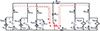 |
Fig. 5 Simplified equivalent steady-state circuit model of a DC microgrid. |
3 Fault detection approach
The discharging capacitors in DCMG respond rapidly to DC-link faults. Their dynamic behaviour is exploited for fault detection, as the capacitor current exhibits a peak spike towards the fault [75, 76]. The peak current magnitude depends on the fault type and location. DER and battery jth capacitors discharge their stored energy  during a transient period before reaching zero in a steady state. For a constant 90 V across Ci, the power in Cj is similarly determined. Despite the RC circuit configuration, power dissipates through a resistive path associated with Cj. Generally, the peak discharge current depends on RCeqj, when the discharge current is expressed as
  . The peak discharge current reflects the fault type, as it’s influenced by the equivalent resistance of parallel loads, cables, and fault resistance [77, 78]. In this method, comparing the current patterns from the capacitor under dynamic conditions is essential to locate the fault accurately.
 where RC is the cable (line) resistance, RLj is the resistance of the different load zones (i.e., Rl1, Rl2, Rl3, Rl4, Rl5, and Rl6), and Rf is the fault resistance.
Figure 6 shows the flowchart for the proposed fault detection and location method. The algorithm starts with the RS setup, after which the RS exclusively collect the capacitor currents iCj|j = iC1 − iC5. The process involves sampling, averaging the sample flows, and calculating fault indices. The detailed flowchart steps are given below.
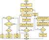 |
Fig. 6 Flowchart of the proposed fault detection and location algorithm. |
3.1 Sampling capacitor currents (iCj)
The Analogue-To-Digital Converter (ADC) samples currents, with (k) and (k − 1) denoting present and previous sampling times. The present and previous average patterns for the ith capacitor currents are given in (5) and (6). The corresponding times are defined as the difference between samples, tk and tk−1. The capacitor current is displayed by the fault equations in load zone 1, which are detailed in Figure 7. The average sample currents for the capacitor iC1 are represented by  and
and  (k − 1).
 (5)
(5)
 (6)
(6)
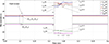 |
Fig. 7 Simulation-based validation of the derived equation. |
At fault inception, the equivalent resistance remains constant: RCeqj (k) ≠ RCeqj(k − 1).
3.2 Fault index ( )
)
Equation (7) calculates the fault index “ ”, which represents the difference between consecutive current samples.
 (7)
(7)
 (8)
(8)
At fault initiation, the jth capacitor’s voltage remains constant, Vsj(tk) ≈ Vsj(tk−1) ≈ Vsj with a maintained voltage of 90 V. Therefore, equation (8) can be simplified to equation (9).![Mathematical equation: $$ \delta i_{Cj} = V_{sj} \left[ \frac{1}{R_{Ceqj}(k)} * e^{\left( -t_k R_{Ceqj}(k) * C_j \right)} \right. \\ \left. - \frac{1}{R_{Ceqj}(k-1)} * e^{\left( -t_{k-1} / R_{Ceqj}(k-1) * C_j \right)} \right]. $$](/articles/stet/full_html/2026/01/stet20250193/stet20250193-eq18.gif) (9)
(9)
3.3 Fault detection and characterization
The presented DCMG configuration employs six discharging capacitors, necessitating six RS for capacitor current measurement, crucial for reliable system operation. The proposed fault detection methodology is shown in Figure 6. The process begins by initializing RS states (Sj), where Sj = 1 denotes an active state and Sj = 0 an inactive state, represented by the RS state vector [79, 80]. The RS states are determined through a sampling procedure and transmitted to CBs, ensuring a timely response. Sampled capacitor currents  (k) are averaged to generate present and past sample models,
  (k) and
  (k − 1), for comparative analysis. The fault index (δ
 ) is subsequently calculated using (7), a key metric for fault detection. The RC discharge circuit’s time constant is inversely proportional to fault resistance and directly proportional to peak discharge current [81]. Consequently, LIFs display faster capacitor discharge and higher peak current magnitudes than HIFs, affecting system stability and safety. The decay of iC is exponential at the initial stage of the fault. After the system reaches a steady state, it becomes difficult to isolate the issue, which could have an impact on consumer power quality and grid stability [82, 83]. A detection threshold (δiCth) is defined for each jth capacitor to detect both HIFs and LIFs, ensuring comprehensive protection. Lower and upper characterization thresholds (iCthl and iCthu) are defined based on
  , which is influenced by Rf. Fault resistances (Rf) exceeding 1Ω are classified as HIFs, while those within 0 < Rf < 1 Ω are classified as LIFs [4], reflecting industry standards. This ensures community safety and minimizes disruption.
Analytical analysis using (2) for a 2.3 kW/90 V DCMG reveals maximum capacitor (C1–C5) discharge currents ranging from approximately 28–2 A for fault resistances (Rf1) between 0.1 Ω and 10 Ω. Immediately following a fault, the calculated δiCj surpasses the detection threshold (δiCth) of 0.2 A. The corresponding zone is flagged as faulty when δiCj exceeds δiCth. Based on these findings, the fault characterization threshold (δiCthl) must be 4 A to effectively distinguish between faults and other system disturbances. To minimize misclassification, iCthl and iCthu are set to 2.5 A and 30 A, respectively. If iCj falls below iCthl, a “no-fault” condition is assumed. Conversely, if δiCj exceeds iCthu, a “LIF” is classified. “HIF” detection occurs when δiCj lies between these thresholds. The misclassification index is defined in (10). This approach aims to minimize power interruptions, ensuring community reliance on a stable energy supply. (10)
(10)
3.4 Prediction of fault location in DC microgrid
The fault location method determines fault distance by analysing line data. The estimating line resistance and total line resistance enable fault point distance calculation, as shown in Figure 8. A bus system, with multiple voltage sources supplying fault current δiCj, is used to illustrate the LG fault location algorithm. This ensures efficient power restoration, minimizing disruption in the grid line.![Mathematical equation: $$ \delta {i}_{{Cj}}={V}_{{sj}}\left[\frac{1}{{R}_{{dCeqj}}(k)}*{e}^{\left(-{t}_{k/{R}_{{dCeqj}}(k){*Cj}}\right)}-\frac{1}{{R}_{{dCeqj}}\left(k-1\right)}*{e}^{\left(-{t}_{k-1}/{R}_{{dCeqj}}\left(k-1\right){*Cj}\right)}\right]. $$](/articles/stet/full_html/2026/01/stet20250193/stet20250193-eq25.gif) (11)
(11)
 |
Fig. 8 Simplified equivalent circuit during fault location based on the DC microgrid. |
The above-given equation can be rewritten for fault location prediction.
 (12)∴location-based discharged jth capacitor current is
 (13)
(13)
The determination of the fault distance, denoted as “d”, is achieved through a calculation as (14)where d is the fault distance from any source of the node point bus, dR is RC up to the fault point, R is the DC line segment resistance, and l is the line segment of overall length, respectively. The estimated percentage error of fault location is expressed as
 (15)
(15)
If the fault index difference δiCj exceeds a predetermined threshold (ξ) and the fault distance (d) falls within 0 < d < 1. The algorithm identifies an internal fault, triggering a CB trip signal for protection. The algorithm of the flowchart is shown in Figure 6, voltage and current data are initially received at line segment endpoints from RS. Equation (7) is used to estimate the fault index of the jth capacitor current. If the fault index difference surpasses the threshold, the fault is detected, initiating classification and location procedures. Following the classification, the fault location algorithm commences. In this phase, RS estimate line resistance (R) and fault point resistance (dR) using (13). The fault distance (d) is calculated using the formula (14). This ensures rapid fault mitigation, minimising power disruptions that impact grid well-being.
3.5 Fault isolation process
To pinpoint the fault location between the source and the load, an iterative procedure based on δiCj is employed. It initiates with a RS trip signal (TS = 0, where 0 = off, 1 = on), and the algorithm continuously monitors δiCj. If δiCj remains above iCthl after tripping the RS, it indicates a system fault or a fault in a non-responsive load. The algorithm then deactivates the subsequent RS (TS = 0). If the calculated fault distance falls within 0 < d < 1, the algorithm classifies the fault as internal or external. This iterative process continues until the fault is located. Upon detecting an internal fault, permanent trip signals are sent to all RS, triggering CBs to isolate the fault. This approach minimizes power disruption, ensuring grid safety and maintaining essential services.
3.6 Working of the proposed scheme
Figure 6 shows a flowchart of the proposed algorithm, specifically developed for real-time fault identification and localization in a DCMG based on capacitor current transient dynamics. The algorithm begins with system initialization, where a control flag Sj is assigned the value of 1, indicating an active monitoring state. Following initialization, the algorithm systematically acquires voltage (V) and current (I) values from both the source and load terminals. Simultaneously, it samples capacitor currents iCj(k) at each zone within the DCMG. A key step involves computing the fault index δiCj, which is the difference between the current capacitor sample iCj(k) and its immediate past value iCj(k− 1), thereby detecting transient anomalies. This computed fault index is then compared against a pre-set threshold δiCth. If δiCj > δiCth a possible fault is identified. Subsequently, the nature of the fault is classified by comparing the magnitude of iCj against two characterization thresholds – lower iCthl and upper iCthu – to distinguish between low-impedance and HIFs . Upon confirming a fault, the algorithm proceeds to calculate fault distance (d) by determining the segment resistance (dR) and estimating equivalent resistance dReq. If the computed distance lies within the cable length (0 < d < 1), the algorithm activates a trip signal to isolate the faulted section. If the fault is external or δiCj is below the threshold, the system resets. This real-time scheme enhances protection reliability in DCMGs.
4 Analysis of simulation results and related discussion
4.1 Configuration of the simulation model
Figure 1 shows a DCMG model with an LL-based SC fault simulated in MATLAB/Simulink to evaluate the effectiveness of the proposed fault detection scheme. The system components and parameters are presented in Table 1. A common DC bus connects six loads with a total power of 100 W. Each load zone is powered by a specific source (PV, wind, UG, Bat1, Bat2). The PV and wind converters operate in maximum power point tracking (MPPT) mode, while the battery converter regulates the DC-link voltage at 90 V. The active PV and Battery sources supply 2.32 kW and 253 W, respectively. Although the simulation framework effectively supports fault-detection validation in a realistic DCMG scenario, the results presented lack clarity. The analysis of system behaviour under various fault conditions is insufficient and should be more explicitly addressed to strengthen the study’s impact.
4.2 A computational modelling study
This study examines the proposed algorithm’s performance under various LL SC faults within the simulated DCMG.
1) case 1: Detection of Faults with High Impedance: An LL fault with 9 Ω resistance (Rf1) is introduced near a load in zone 1 at 0.3 ms. Figure 9a displays the resulting load voltage waveforms, illustrating the fault’s impact. This study provides insight into HIF behaviour under specific conditions. The capacitor currents  (k) to
  (k), and their delayed versions
  (k − 1) to
  (k − 1), are shown in Figure 9b, with a TS delay of 40 μs. During fault initiation, capacitors C1–C3 face lower resistance than C4–C5, resulting in higher discharge currents. The δiC1–δiC3 values exceed the threshold δiCth, identifying zone 1 as the fault area. Relay (R1) isolates the fault, de-energizing RL1 (voA = ioA = 0), while other buses are restored within milliseconds. The observed transient signals align with earlier analysis. The iC1–iC3 are classified as HIFs, as their peaks exceed δiCth but not δiCthu. Although the algorithm demonstrates reliable HIF detection and fault isolation. A more detailed explanation of the system’s dynamic response and current behavior under HIF scenarios is needed. Addressing this will enhance the analysis and improve the understanding of the proposed method’s reliability in realistic fault conditions.
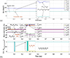 |
Fig. 9 Results during the fault at load zone 1 (a) Bus Voltage. (b) Capacitor current and Trip signal. |
2) Case 2: Detection of Faults with Low Impedance: A similar methodology is applied for LIF detection. An LL fault with resistance (Rf5) of 0.5 Ω is introduced near RL5 in load zone 2. Figure 10 illustrates the resulting bus voltages and capacitor currents. The calculated δiC4–δiC5 values exceed the threshold δith, while δiC1–δiC3 remain below it, confirming zone 2 as the fault location and isolating RL5. The LIF condition is validated by iC3 exceeding δiCthu. The algorithm’s selectivity is evident as the fault index remains below ithl during load variations, preventing false trips. However, the clarity of these results remains limited, making it difficult to interpret the capacitor current behavior during LIF events. A more detailed analysis is needed to effectively demonstrate the algorithm’s robustness under varying fault conditions.
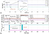 |
Fig. 10 Results during the fault at load zone 2 (a) Bus Voltage. (b) Capacitor current and Trip signal. |
The capacitor current dynamics (C4–C5) during LIF (Rf5 = 0.5 Ω) LL faults in load zones 1 and 2 are depicted in Figures 11a and 11b, demonstrating the algorithm’s ability to distinguish between fault locations. In both figures, Q1–Q3 represents capacitor currents (iC1–iC5) before and after steady-state faults. At time t₁, a fault in load zone 1 causes C1–C3 to encounter higher resistance than C4–C5, resulting in lower peak discharge currents for iC1–iC3 than iC4–iC5. At time  , a fault in zone 2 creates lower resistance at C4–C5, leading to a higher discharge peak than iC1–iC3. This confirms the algorithm’s ability to identify fault zones by analyzing peak capacitor currents during transient conditions. The scheme also supports fast detection; for instance, an LIF with Rf1 = 9 Ω near RL1 is identified by sensing capacitor current at t1. The corresponding fault index δiCj is computed using algorithm (6), validating the method’s performance in real-time detection and localization. However, while the results suggest accurate operation, the explanation lacks clarity. A more detailed analytical interpretation of the capacitor behavior under different fault cases is needed to clearly support the claimed robustness of the proposed method.
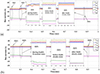 |
Fig. 11 Capacitor currents (iC1 − iC5) behavior during a low-impedance LL fault. (a) At t1 A fault occurred in load zone 1 near RL1. (a) At t2 A fault occurred in load zone 2 near RL5. |
4.3 EV state during charge level and non-faulty variations.
The proposed algorithm’s safety is evaluated during EV charger activation on a DCMG bus, with the initial EV charge state set at 20%. The RS current measurements are shown in Figure 11. Due to the high inrush current of the EV charger, conventional overcurrent protection proves less effective in DCMGs. However, the proposed algorithm consistently ensures reliable fault detection during EV charger switching, demonstrating robustness against dynamic load variations, secure operation, and prevention of false trips. This reinforces DCMG security during EV charging, a vital aspect of grid stability. Figure 12 illustrates the dynamic response of a non-faulty load during remote fault conditions. At 0.3 ms, faults at RL1 (9 Ω) and RL5 (0.5 Ω) trigger isolation. The TS isolates the fault, as reflected in switch state transitions. The no-faulty load voltage (VOC) shows a transient dip but quickly returns to nominal, confirming voltage resilience. Similarly, the capacitor current (ICload) for the non-faulty load spikes and then stabilizes, indicating current regulation. Although the results demonstrate fault-handling capabilities, the reviewer observes a lack of clarity in the presentation. The explanation of system dynamics during EV charging and non-faulty load responses requires further analytical depth to better validate the algorithm’s effectiveness under such operating conditions.
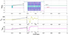 |
Fig. 12 Contribution of the capacitor for nonfaulty load, i.e., RL3. |
4.4 DC Microgrid operation under fluctuating generation conditions
To assess the algorithm’s performance under variable generation conditions, the irradiance of a PV panel connected to a DC bus is increased by 25% within 0.3 s. This results in a corresponding increase in the load output voltage at 0.3 s, as shown in Figure 13a. The DERs of capacitive currents measured at all sources, batteries, and also trip signals, are shown in Figure 13b. The proposed method maintains its security during these variable generation scenarios in the DCMG, demonstrating its robustness against fluctuating power inputs. However, the explanation lacks clarity, and the analysis of the system’s transient behavior under such variations needs to be expanded to better validate the algorithm’s effectiveness and reliability.
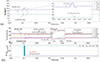 |
Fig. 13 Results during the changes of DERs (a) Bus Voltage. (b) Capacitor current and Trip signal. |
4.5 Precise fault location
The accuracy of the proposed fault location methodology is evaluated by simulating LL faults (Rf1 and Rf2) on the line segment, varying both fault distance (d) and fault resistance (Rf). Fault distance predictions are performed at RS positioned between source and load locations using the proposed approach. The positional errors in fault estimation are quantified and presented in Table 2. Results indicate that the maximum error using the proposed fault distance prediction method is 2.59%, validating its capability to provide accurate fault location, critical for efficient fault clearance and minimizing downtime in DCMG systems.
Comparative analysis of fault detection and location methods.
Figures 14a and 15a show the voltage profiles of the source and load during fault conditions. Figures 14b and 15b illustrate the respective current responses. Figures 14c and 15c display the calculated line resistance (R) and fault resistances (Rf1, Rf2) up to the fault location (dR). Figures 14d and 15d present the corresponding fault distances within 1 p.u. for LL faults. These calculations confirm the successful identification of internal faults and prompt activation of trip signals at the appropriate CB. However, while the results indicate promising accuracy, the supporting analysis lacks depth. A more detailed explanation of the resistance estimation and fault location logic is needed for clarity.
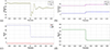 |
Fig. 14 L-L fault (Rf1) of the DCMG (a) Voltages of source and fault load. (b) Currents of source and fault load. (c) Estimated resistance. (d) Fault distance. |
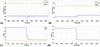 |
Fig. 15 L-L fault (Rf2) of the DCMG (a) Voltages of source and fault load. (b) Currents of source and fault load. (c) Estimated resistance. (d) Fault distance. |
4.6 Comparative analysis
Table 2 compares the proposed technique with various existing fault detection and location methods in DCMG. The comparison is based on several parameters, including the type of sensing variable, fault resistance, fault detection time, fault location, and estimated errors. The proposed technique utilizes capacitor current (C–C) as the sensing variable and can detect faults with a resistance of up to 10 Ω. It has a fault detection time of 2.3 ms and can locate faults on the load side (LS) with an estimated error of 2.59%. Compared to past methods, such as those relying on line current (L–C), line voltage (L–V), or filter capacitor current (FC–C), which either lacked fault classification or had higher detection time and location errors, the proposed method offers superior detection sensitivity and accuracy. Many previous techniques were limited to specific conditions or required complex hardware, whereas the proposed scheme achieves effective detection with minimal overhead. Thus, Table 2 highlights a clear improvement in fault management performance by the proposed approach.
A pie chart is used to visualize this comparative analysis in Figure 16. The chart divides parameters into segments, with section sizes proportional to their respective values. It illustrates the share of methods using different sensing variables (C–C, FC–C, L–C, etc.) and reflects trends in detection times. Analytical observation confirms that C-C-based methods dominate due to their balance of speed and reliability. The chart also reveals limitations in earlier techniques, such as a lack of classification or high error rates. In contrast, the proposed method integrates fast detection, fault classification, and accurate location. Overall, the visual analysis reinforces the proposed technique’s advantage over prior work by demonstrating enhanced robustness, reliability, and suitability for modern DCMGs with renewable integration.
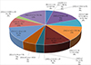 |
Fig. 16 A comparative study between the newly developed technique and existing protective measures. |
5 Conclusion
This paper presents a novel SC fault detection and location technique for renewable energy-integrated DCMG. Employing CBs in conjunction with RS. The algorithm determines fault locations by comparing line segment energy profiles. Fault zone identification is achieved through analyzing capacitor current dynamics during LL SC faults. The method estimates fault distances by calculating line and fault point resistances, demonstrating robustness under variable generation and fault scenarios. Comparative assessments reveal the proposed scheme’s enhanced performance compared to existing fault detection and localization methods. This contributes to improved reliability and resilience in DCMG systems, ensuring efficient fault management and minimizing downtime in renewable-based DCMGs.
Funding
The authors did not receive any funding.
Conflicts of interest
Authors do not have any conflicts.
Author contribution statement
Banothu Somanna has designed the framework, analyzed performance, validated the results, and written the article. Sushma Gupta has collected the information required for the framework, provided software, conducted critical reviews, and administered the process.
Ethics approval
Does not involve any studies with animals or humans.
References
- Patterson B.T. (2012) DC, come home: DC microgrids and the birth of the "Enernet", IEEE Power Energy Mag. 10, 6, 60–69. [Google Scholar]
- Committee E.M. (1992) IEEE Recommended Practice for Monitoring, Vol. 2004. [Google Scholar]
- Dragičević T., Lu X., Vasquez J.C., Guerrero J.M. (2016) DC microgrids-Part II: A review of power architectures, applications, and standardization issues, IEEE Trans. Power Electron. 31, 5, 3528–3549. [Google Scholar]
- Bhargav R., Bhalja B.R., Gupta C.P. (2020) Novel fault detection and localization algorithm for low voltage DC microgrid, IEEE Trans. Ind. Informat. 16, 7, 4498–4511. [Google Scholar]
- Rao G.K., Jena P. (2023) A novel fault identification and localization scheme for bipolar DC microgrid, IEEE Trans. Ind. Informat. 19, 12, 11752–11764. [Google Scholar]
- Salomonsson D., Soder L., Sannino A. (2009) Protection of low-voltage DC microgrids, IEEE Trans. Power Delivery 24, 3, 1045–1053. [Google Scholar]
- Yang J., Fletcher J.E., O'Reilly J. (2012) Short-circuit and ground fault analyses and location in VSC-based DC network cables, IEEE Trans. Ind. Informat. 59, 10, 3827–3837. [Google Scholar]
- Maqsood A., Corzine K. (2016) DC Microgrid Protection: Using the Coupled-Inductor Solid-State Circuit Breaker, IEEE Electrific. Mag. 4, 2, 58–64. [Google Scholar]
- Cairoli P., Dougal R.A., Ghisla U., Kondratiev I. (2010) Power sequencing approach to fault isolation in dc systems: Influence of system parameters, in: 2010 IEEE Energy Conversion Congress and Exposition, pp. 72–78. [Google Scholar]
- Meghwani A., Chakrabarti S., Srivastava S.C., Anand S. (2017) Analysis of fault characteristics in DC microgrids for various converter topologies, in: 2017 IEEE Innovative Smart Grid Technologies – Asia (ISGT-Asia), pp. 1–6. [Google Scholar]
- Yu M., Wang Y., Zhang L., Zhang Z. (2016) DC short circuit fault analysis and protection of ring type DC microgrid, in: 2016 IEEE 8th International Power Electronics and Motion Control Conference (IPEMC-ECCE Asia), 1694–1700. [Google Scholar]
- Jamshidpour E., Poure P., Saadate S. (2015) Photovoltaic systems reliability improvement by real-time FPGA-based switch failure diagnosis and fault-tolerant DC–DC converter, IEEE Trans. Ind. Informat. 62, 11, 7247–7255. [Google Scholar]
- Yadav N., Tummuru N.R. (2023) Application of filter capacitor dynamics based short-circuit fault detection method in ring-type DC microgrid, IEEE Trans. Ind. Informat. 70, 5, 5286–5295. [Google Scholar]
- Tang L., Ooi B.-T. (2007) Locating and isolating DC faults in multi-terminal DC systems, IEEE Trans. Power Delivery 22, 3, 1877–1884. [Google Scholar]
- Dhar S., Patnaik R.K., Dash P.K. (2018) Fault detection and location of photovoltaic based DC microgrid using differential protection strategy, IEEE Trans. Smart Grid, 9, 5, 4303–4312. [Google Scholar]
- Meghwani A., Gokaraju R., Srivastava S.C., Chakrabarti S. (2020) Local measurements-based backup protection for DC microgrids using sequential analyzing technique, IEEE Syst. J. 14, 1, 1159–1170. [Google Scholar]
- Som S., Samantaray S.R. (2018) Efficient protection scheme for low-voltage DC micro-grid, IET Gener. Transmiss. Distrib. 12, 13, 3322–3329. [Google Scholar]
- Fletcher S.D.A., Norman P.J., Fong K., Galloway S.J., Burt G.M. (2014) High-speed differential protection for smart DC distribution systems, IEEE Trans. Smart Grid 5, 5, 2610–2617. [Google Scholar]
- Meghwani A., Srivastava S.C., Chakrabarti S. (2017) A non-unit protection scheme for DC microgrid based on local measurements, IEEE Trans. Power Delivery 32, 1, 172–181. [Google Scholar]
- Christopher E., Sumner M., Thomas D.W.P., Wang X., de Wildt F. (2013) Fault location in a zonal DC marine power system using active impedance estimation, IEEE Trans, Ind. Appl. 49, 2, 860–865. [Google Scholar]
- Cairoli P., Dougal R.A. (2018) Fault detection and isolation in medium-voltage DC microgrids: Coordination between supply power converters and bus contactors, IEEE Trans. Power Electron. 33, 5, 4535–4546. [Google Scholar]
- Yadav N., Tummuru N.R. (2022) Short-circuit fault detection and isolation using filter capacitor current signature in low-voltage DC microgrid applications, IEEE Trans. Ind. Informat. 69, 8, 8491–8500. [Google Scholar]
- Saleh K.A., Hooshyar A., El-Saadany E.F. (2017) Hybrid passive-overcurrent relay for detection of faults in low-voltage DC grids, IEEE Trans. Smart Grid 8, 3, 1129–1138. [Google Scholar]
- Yeap Y.M., Geddada N., Satpathi K., Ukil A. (2018) Time- and frequency-domain fault detection in a VSC-interfaced experimental DC test system, IEEE Trans. Ind. Inform. 14, 10, 4353–4364. [Google Scholar]
- Baran M.E., Mahajan N.R. (2007) Overcurrent protection on voltage-source-converter-based multiterminal DC distribution systems, IEEE Trans. Power Delivery 22, 1, 406–412. [Google Scholar]
- Emhemed A.A.S., Fong K., Fletcher S., Burt G.M. (2017) Validation of fast and selective protection scheme for an LVDC distribution network, IEEE Trans. Power Delivery 32, 3, 1432–1440. [Google Scholar]
- Mohanty R., Pradhan A.K. (2018) Protection of smart DC microgrid with ring configuration using parameter estimation approach, IEEE Trans. Smart Grid 9, 6, 6328–6337. [Google Scholar]
- Rao G.K., Jena P. (2022) Fault detection in DC microgrid based on the resistance estimation, IEEE Syst. J. 16, 1, 1009–1020. [Google Scholar]
- Saxena A., Sharma N.K., Samantaray S.R. (2022) An enhanced differential protection scheme for LVDC microgrid, IEEE J. Emerging Selected Topics Power Electron. 10, 2, 2114–2125. [Google Scholar]
- Jarrahi M.A., Samet H., Ghanbari T. (2023) Fault detection in DC microgrid: A transient monitoring function-based method, IEEE Trans. Ind. Informat. 70, 6, 6284–6294. [Google Scholar]
- Srivastava C., Tripathy M. (2023) Novel adaptive fault detection strategy in DC microgrid utilizing statistical-based method, IEEE Trans. Ind. Inform. 19, 5, 6917–6929. [Google Scholar]
- Yang Y., Huang C., Xu Q. (2020) A fault location method suitable for low-voltage DC line, IEEE Trans. Power Delivery 35, 1, 194–204. [Google Scholar]
- Narasipuram R.P., Pasha M.M., Tabassum S., Tandon A.S. (2025) The electric vehicle surge: effective solutions for charging challenges with advanced converter technologies, Energy Eng. 122, 2, 431–469. [CrossRef] [Google Scholar]
- Narasipuram R.P., Mopidevi S. (2024) Assessment of E-mode GaN technology, practical power loss, and efficiency modelling of iL2C resonant DC-DC converter for xEV charging applications, J. Energy Storage, 91, 112008. [Google Scholar]
- Narasipuram R. (2024) A novel high step-up DC–DC converter using state space modelling technique for battery storage applications, Clean Energy Sustain. 2, 10003. [Google Scholar]
- Abdali A., Mazlumi K., Noroozian R. (2019) High-speed fault detection and location in DC microgrids systems using multi-criterion system and neural network, Appl. Soft Comput. J. 79, 341–353. [Google Scholar]
- Park J.-D., Candelaria J., Ma L., Dunn K. (2013) DC ring-bus microgrid fault protection and identification of fault location, IEEE Trans. Power Delivery 28, 4, 2574–2584. [Google Scholar]
- Kong L., Nian H. (2021) Fault detection and location method for mesh-type DC microgrid using pearson correlation coefficient, IEEE Trans. Power Delivery 36, 3, 1428–1439. [Google Scholar]
- Yalavarthy U.R.S., Kumar N.B., Babu A.R.V., Narasipuram R.P., Padmanaban S. (2025) Digital twin technology in electric and self-navigating vehicles: Readiness, convergence, and future directions, Energy Convers. Manag. 26, 100949. [Google Scholar]
- Narasipuram R.P., Mopidevi S. (2024) Steady-state and transient analysis of LLC and iLLC resonant DC–DC converters with wide voltage operations using GaN technology for light-duty xEV charging systems, Energy Technol. 13, 8, 2400506. [Google Scholar]
- Vijay Babu A.R., Bharath Kumar N., Patnaik Narasipuram R., Periyannan S., Hosseinpour A., Flah A. (2025) Solar energy forecasting using machine learning techniques for enhanced grid stability, IEEE Access 13, 93735–93754. [Google Scholar]
- Geddada N., Yeap Y.M., Ukil A. (2018) Experimental validation of fault identification in VSC-based DC grid system, IEEE Trans. Ind. Informat. 65, 6, 4799–4809. [Google Scholar]
- Tong A., Zhang J., Xie L. (2024) Intelligent fault diagnosis of rolling bearing based on gramian angular difference field and improved dual attention residual network, Sensors 24, 7, 2156. 10.3390/s24072156 [CrossRef] [PubMed] [Google Scholar]
- Wang Q., Chen L., Xiao G., Wang P., Gu Y., Lu J. (2024) Elevator fault diagnosis based on digital twin and PINNs-e-RGCN, Scientific Rep. 14, 1, 30713. 10.1038/s41598-024-78784-7 [Google Scholar]
- Ma K., Yang J., Liu P. (2020) Relaying-assisted communications for demand response in smart grid: cost modeling, game strategies, and algorithms, IEEE J. Selected Areas Commun. 38, 1, 48–60. 10.1109/JSAC.2019.2951972 [Google Scholar]
- Zhang J., Feng X., Zhou J., Zang J., Wang J., Shi G., Li Y. (2023) Series-shunt multiport soft normally open points, IEEE Trans. Ind. Informat. 70, 11, 10811–10821. 10.1109/TIE.2022.3229375 [Google Scholar]
- Li Y., Song L., Hu Y., Lee H., Wu D., Rehm P.J., Lu N. (2024) Load profile inpainting for missing load data restoration and baseline estimation, IEEE Trans. Smart Grid 15, 2, 2251–2260. 10.1109/TSG.2023.3293188 [Google Scholar]
- Li N., Zhang C., Liu Y., Zhuo C., Liu M., Yang J., Zhang Y. (2024) Single-degree-of-freedom hybrid modulation strategy and light-load efficiency optimization for dual-active-bridge converter, IEEE J. Emerging Selected Topics Power Electron. 12, 4, 3936–3947. 10.1109/JESTPE.2024.3396340 [Google Scholar]
- Li N., Cao Y., Liu X., Zhang Y., Wang R., Jiang L., Zhang X. (2024) An improved modulation strategy for single-phase three-level neutral-point-clamped converter in critical conduction mode, J. Modern Power Syst. Clean Energy 12, 3, 981–990. 10.35833/MPCE.2023.000210 [Google Scholar]
- Zhi S., Su K., Yu J., Li X., Shen H. (2025) An unsupervised transfer learning bearing fault diagnosis method based on multi-channel calibrated transformer with shiftable window, Structural Health Monitoring. 10.1177/14759217251324671 [Google Scholar]
- Zeng Z., Goetz S.M. (2024) A general interchanged interleaving carriers for eliminating DC/low-frequency circulating currents in multiparallel three-phase power converters, IEEE Trans. Power Electron. 39, 10, 12323–12335. 10.1109/TPEL.2024.3407207 [Google Scholar]
- Zeng Z., Goetz S.M. (2025) A zero common mode voltage PWM scheme with minimum zero-sequence circulating current for two-parallel three-phase two-level converters, IEEE J. Emerging Selected Topics Power Electron. 13, 2, 1503–1513. 10.1109/JESTPE.2024.3409290 [Google Scholar]
- Saleh K.A., Hooshyar A., El-Saadany E.F. (2019) Ultra-high-speed traveling-wave-based protection scheme for medium-voltage DC microgrids, IEEE Trans. Smart Grid 10, 2, 1440–1451. [Google Scholar]
- Zhang J., Ji Y., Zhou J., Jia Y., Shi G., Wang H. (2025) Cooperative AC/DC voltage margin control for mitigating voltage violation of rural distribution networks with interconnected DC link, IEEE Trans. Power Delivery 40, 2, 1014–1029. 10.1109/TPWRD.2025.3535712 [Google Scholar]
- Zhang S., He Y., Gu Y., He Y., Wang H., Wang H., Zhou B. (2025) UAV based defect detection and fault diagnosis for static and rotating wind turbine blade: A review, Nondestruct. Test. Eval. 40, 4, 1691–1729. 10.1080/10589759.2024.2395363 [Google Scholar]
- Xu X., Deng J., Lin H., Li Z., Wen H. (2025) Lightweight anomalous detection of hydro turbine operation sound using fusion network enhanced by load information, IEEE Trans. Instrum. Meas. 74, 1–13. 10.1109/TIM.2025.3533632 [Google Scholar]
- Wang S., Cheng Q., Shangguan B., Ma J., Jiao N., Liu T. (2025) Accurate and continuous reactive power control of three-terminal hybrid DC transmission system, IEEE Trans. Power Delivery 40, 1, 30–40. 10.1109/TPWRD.2024.3480270 [Google Scholar]
- Wang J., Song Y., He T. (2025) A novel adaptive monitoring framework for detecting the abnormal states of aero-engines with maneuvering flight data, Reliab. Eng. Syst. Safety 258, 110910. 10.1016/j.ress.2025.110910 [Google Scholar]
- Liu F., Zhao X., Zhu Z., Zhai Z., Liu Y. (2023) Dual-microphone active noise cancellation paved with Doppler assimilation for TADS, Mech. Syst. Signal Process. 184, 109727. 10.1016/j.ymssp.2022.109727 [Google Scholar]
- Yang Y., Zhang Z., Zhou Y., Wang C., Zhu H. (2023) Design of a simultaneous information and power transfer system based on a modulating feature of magnetron, IEEE Trans. Microw. Theory Tech. 71, 2, 907–915. 10.1109/TMTT.2022.3205612 [Google Scholar]
- Li N., Wang H. (2025) Variable filtered-waveform variational mode decomposition and its application in rolling bearing fault feature extraction, Entropy 27, 3, 277. 10.3390/e27030277 [Google Scholar]
- Lin L., Liu J., Huang N., Li S., Zhang Y. (2024) Multiscale spatio-temporal feature fusion based non-intrusive appliance load monitoring for multiple industrial industries, Appl. Soft Comput. 167, 112445. 10.1016/j.asoc.2024.112445 [CrossRef] [Google Scholar]
- Zhang C., Qiao J., Wang S., Chen R., Dui H., Zhang Y., Zhou Y. (2025) Importance measures based on system performance loss for multi-state phased-mission systems, Reliab. Eng. Syst. Safety 256, 110776. 10.1016/j.ress.2024.110776 [Google Scholar]
- Subramaniam K., Illindala M.S. (2020) Intelligent three tie contactor switch unit-based fault detection and isolation in DC microgrids, IEEE Trans. Ind. Appl. 56, 1, 95–105. [Google Scholar]
- Lee W.-S., Kim J.-H., Lee J.-Y., Lee I.-O. (2019) Design of an isolated DC/DC topology with high efficiency of over 97% for EV fast chargers, IEEE Trans. Vehicular Technol. 68, 12, 11725–11737. [Google Scholar]
- Zhang X., Gong C. (2013) Dual-buck half-bridge voltage balancer, IEEE Trans. Ind. Informat. 60, 8, 3157–3164. [Google Scholar]
- Scheiterer R.L., Na C., Obradovic D., Steindl G. (2009) Synchronization performance of the precision time protocol in industrial automation networks, IEEE Trans. Instrum. Meas. 58, 6, 1849–1857. [Google Scholar]
- Somanna B., Gupta S. (2025) Enhancing reliability and resilience in AC/DC hybrid microgrids: A unified fault detection and control approach with optimized-tuned PI controller for UPQC, SN Comput. Sci. 6, 247. [Google Scholar]
- Rong Q., Hu P., Wang L., Li Y., Yu Y., Wang D., Cao Y. (2024) Asymmetric sampling disturbance-based universal impedance measurement method for converters, IEEE Trans. on Power Electron. 39, 12, 15457–15461. 10.1109/TPEL.2024.3451403 [Google Scholar]
- Liu K., Jiao S., Nie G., Ma H., Gao B., Sun C., Wu G. (2024) On image transformation for partial discharge source identification in vehicle cable terminals of high-speed trains, High Voltage 9, 5, 1090–1100. 10.1049/hve2.12487 [CrossRef] [Google Scholar]
- Gao S., Chen Y., Song Y., Yu Z., Wang Y. (2024) An efficient half-bridge MMC model for EMTP-type simulation based on hybrid numerical integration, IEEE Trans. Power Syst. 39, 1, 1162–1177. 10.1109/TPWRS.2023.3262584 [CrossRef] [Google Scholar]
- Wang X., Wang H., Peng M. (2025) Interpretability study of a typical fault diagnosis model for nuclear power plant primary circuit based on a graph neural network, Reliab. Eng. Syst. Safety 261, 111151. 10.1016/j.ress.2025.111151 [Google Scholar]
- Wang H., Li Y., Men T., Li L. (2024) Physically interpretable wavelet-guided networks with dynamic frequency decomposition for machine intelligence fault prediction, IEEE Trans. Syst., Man Cybernetics Syst. 54, 8, 4863–4875. 10.1109/TSMC.2024.3389068 [Google Scholar]
- Meng Q., Hussain S., Luo F., Wang Z., Jin X. (2025) An online reinforcement learning-based energy management strategy for microgrids with centralized control, IEEE Trans. Ind. Appl. 61, 1, 1501–1510. 10.1109/TIA.2024.3430264 [Google Scholar]
- Lu G., Lin Q., Zheng D., Zhang P. (2025) Online degradation fault prognosis for DC-link capacitors in multistring-connected photovoltaic boost converters subject to cable uncertainties, IEEE J. Emerging Selected Topics Power Electron. 13, 1, 1107–1117. 10.1109/JESTPE.2024.3502255 [Google Scholar]
- Liu L., Li Z., Kang H., Xiao Y., Sun L., Zhao H., Ma Y. (2025) Review of surrogate model assisted multi-objective design optimization of electrical machines: New opportunities and challenges, Renew. Sustain. Energy Rev. 215, 115609. 10.1016/j.rser.2025.115609 [CrossRef] [Google Scholar]
- Wang H., Wang Y., Xiao X., Ma Z., Xu Q. (2025) Harmonic state space based stability analysis of LCC-HVDC system with saturated transformer, IEEE Trans. Power Delivery 40, 4, 2254–2266. 10.1109/TPWRD.2025.3575065 [Google Scholar]
- Wang Y., Chen S., Yang M., Liao P., Xiao X., Xie X., Li Y. (2025) Low-frequency oscillation in power grids with virtual synchronous generators: A comprehensive review, Renew. Sustain. Energy Rev. 207, 114921. 10.1016/j.rser.2024.114921 [Google Scholar]
- Wan A., Zhang F., AL-Bukhaiti K., Cheng X., Ji X., Wang J., Shan T. (2025) A novel GA-PSO-SVM model for compound fault diagnosis in gearboxes with limited data, IEEE Sensors J. 25, 16, 303431–30443. 10.1109/JSEN.2025.3576761 [Google Scholar]
- Wan A., Gong W., Iqbal A., AL-Bukhaiti K., Ji Y., Duer S., Yao F. (2025) Robust loop shaping design pitch control of wind turbine for maximal power output and reduced loading, Energy 319, 135136. 10.1016/j.energy.2025.135136 [Google Scholar]
- Yang M., Jiang R., Yu X., Wang B., Su X., Ma C. (2025) Extraction and application of intrinsic predictable component in day-ahead power prediction for wind farm cluster, Energy 328, 136530. 10.1016/j.energy.2025.136530 [Google Scholar]
- Yang M., Guo Y. (2023) Wind power cluster ultra-short-term prediction error correction method based on the load peak and valley characteristics, CSEE J. Power Energy Syst. 12, 1, 258–270. 10.17775/CSEEJPES.2022.06180 [Google Scholar]
- Bian Y., Xie L., Ma L., Cui C. (2025) A novel two-stage energy sharing model for data center cluster considering integrated demand response of multiple loads, Appl. Energy 384, 125454. 10.1016/j.apenergy.2025.125454 [Google Scholar]
All Tables
All Figures
|
Fig. 1 Schematic diagram of a DC microgrid along with different types of DERs and loads. |
| In the text | |
|
Fig. 2 Equivalent circuit for a LL SC fault in the load zone of the DC microgrid. |
| In the text | |
|
Fig. 3 A simplified equivalent circuit model of the DC microgrid. |
| In the text | |
|
Fig. 4 Simplified equivalent transient-state circuit model of a DC microgrid. |
| In the text | |
|
Fig. 5 Simplified equivalent steady-state circuit model of a DC microgrid. |
| In the text | |
|
Fig. 6 Flowchart of the proposed fault detection and location algorithm. |
| In the text | |
|
Fig. 7 Simulation-based validation of the derived equation. |
| In the text | |
|
Fig. 8 Simplified equivalent circuit during fault location based on the DC microgrid. |
| In the text | |
|
Fig. 9 Results during the fault at load zone 1 (a) Bus Voltage. (b) Capacitor current and Trip signal. |
| In the text | |
|
Fig. 10 Results during the fault at load zone 2 (a) Bus Voltage. (b) Capacitor current and Trip signal. |
| In the text | |
|
Fig. 11 Capacitor currents (iC1 − iC5) behavior during a low-impedance LL fault. (a) At t1 A fault occurred in load zone 1 near RL1. (a) At t2 A fault occurred in load zone 2 near RL5. |
| In the text | |
|
Fig. 12 Contribution of the capacitor for nonfaulty load, i.e., RL3. |
| In the text | |
|
Fig. 13 Results during the changes of DERs (a) Bus Voltage. (b) Capacitor current and Trip signal. |
| In the text | |
|
Fig. 14 L-L fault (Rf1) of the DCMG (a) Voltages of source and fault load. (b) Currents of source and fault load. (c) Estimated resistance. (d) Fault distance. |
| In the text | |
|
Fig. 15 L-L fault (Rf2) of the DCMG (a) Voltages of source and fault load. (b) Currents of source and fault load. (c) Estimated resistance. (d) Fault distance. |
| In the text | |
|
Fig. 16 A comparative study between the newly developed technique and existing protective measures. |
| In the text | |
Current usage metrics show cumulative count of Article Views (full-text article views including HTML views, PDF and ePub downloads, according to the available data) and Abstracts Views on Vision4Press platform.
Data correspond to usage on the plateform after 2015. The current usage metrics is available 48-96 hours after online publication and is updated daily on week days.
Initial download of the metrics may take a while.