")
")
| Issue |
Sci. Tech. Energ. Transition
Volume 80, 2025
Innovative Strategies and Technologies for Sustainable Renewable Energy and Low-Carbon Development
|
|
|---|---|---|
| Article Number | 42 | |
| Number of page(s) | 15 | |
| DOI | https://doi.org/10.2516/stet/2025023 | |
| Published online | 09 June 2025 | |
Regular Article
Energy optimization through morphing blade design under structural constraints: a case study on the NREL 1.5 MW wind turbine
Department of Aerospace Engineering, Amirkabir University of Technology (Tehran Polytechnic), No. 350, Hafez Street, Valiasr Square, Tehran 15875-4413, Iran
* Corresponding author: This email address is being protected from spambots. You need JavaScript enabled to view it.
Received:
4
December
2024
Accepted:
6
May
2025
Abstract
This study explores a novel morphing blade design methodology to enhance the aerodynamic performance of the NREL 1.5 MW wind turbine while addressing structural constraints. The proposed approach applies targeted morphing to the leading and trailing edges of the blade sections, utilizing a streamlined parameterization framework with four shape variables per airfoil: two deflection angles and two deformation starting points. The morphing process is modeled using an m-degree shape function and optimized through a Genetic Algorithm (GA) to maximize power generation while minimizing structural displacement and thrust forces. Turbine performance is initially assessed using Blade Element Momentum (BEM) theory and validated through high-fidelity Computational Fluid Dynamics (CFD) simulations based on the Reynolds-Averaged Navier–Stokes (RANS) equations and the k-ω turbulence model. Results demonstrate significant power coefficient improvements of up to 23.8%, 10%, and 7% at wind speeds of 11.5 m/s, 8 m/s, and 4 m/s, respectively, compared to the baseline configuration. These findings underline the potential of morphing blade technologies to enhance energy efficiency in wind turbines while adhering to practical structural limitations.
Key words: Horizontal-axis wind turbine / Morphing blade / Computational Fluid Dynamics (CFD) / Genetic algorithm optimization / Power coefficient / Structural constraints
© The Author(s), published by EDP Sciences, 2025
 This is an Open Access article distributed under the terms of the Creative Commons Attribution License (https://creativecommons.org/licenses/by/4.0), which permits unrestricted use, distribution, and reproduction in any medium, provided the original work is properly cited.
Aerodynamic parameters
Cp: Power coefficient (–)
CL: Lift coefficient (–)
CD: Drag coefficient (–)
T : Thrust force (N)
α : Angle of attack (°)
ρ : Air density (kg/m3)
λ: Tip speed ratio (–)
V∞: Free-stream wind velocity (m/s)
θ : Maximum displacement angle (°)
τij : Reynolds stress tensor (–)
ν: Kinematic viscosity (m2/s)
A, B, C, D, α : Coefficients in Penalty Functions (–)
Blade and wind turbine parameters
R : Rotor radius (m)
ω : Rotational speed (rpm)
H : Hub height (m)
N : Number of blade elements (–)
C : Chord length (m)
β : Twist angle (°)
x0: Starting point of deflection (m)
η : Transform value in the y-direction (m)
ξ : Non-dimensional length in the x-direction (–)
Morphing blade parameters
MLE: Morphing Leading Edge (–)
MTE: Morphing Trailing Edge (–)
xMLE: Starting point of MLE deformation (m)
xMTE: Starting point of MTE deformation (m)
θMLE: Deflection angle of MLE (°)
θMTE: Deflection angle of MTE (°)
S818: Section of blade using S818 airfoil (–)
S825: Section of blade using S825 airfoil (–)
S826: Section of blade using S826 airfoil (–)
Computational and optimization methods
BEM: Blade Element Momentum (–)
CFD: Computational Fluid Dynamics (–)
SST: Shear Stress Transport (–)
GA: Genetic Algorithm (–)
RANS: Reynolds-Averaged Navier–Stokes (–)(–)
k-ω : Turbulence model (–)
Y + : Non-dimensional wall distance (–)
1 Introduction
Recently, wind energy has become more competitive than nonrenewable sources due to advancements in larger and more durable blades, developed through novel efficiency-enhancing methods. By 2050, its contribution to global power generation is projected to increase from 5% to 30% [1, 2]. One major challenge in wind energy, as seen in the power-speed diagram of wind turbines, is the nonlinear relationship between wind power and speed, preventing turbines from reaching optimal efficiency below the rated speed [2]. However, advanced control techniques have significantly improved power generation and performance while reducing structural loads on wind turbines. Some research has explored the design of flow control systems that contain power control and aerodynamic forces [3]. These technologies have enabled the development of robust, reliable, and cost-effective blades and wind turbine controllers, facilitating a fully automated system. These strategies are classified as active or passive control [4]. The use of active control techniques requires secondary power sources or external energy and may include one or more moving elements positioned on the blade of a wind turbine [5, 6]. Active flow control devices include morphing flaps, stall ribs, synthetic jets, plasma actuators, and especially pitch control systems that manage turbine revolution as a wind velocity function [7]. In contrast, passive control does not require external power, usually installed as stationary parts on the turbine like vortex generators, microtabs, serrated trailing edges, flow vanes, gurney flaps, fixed leading edge slats, airfoils with protuberances, and cavities [8, 9]. Active control of wind turbines seeks to enhance power output through adaptable blade structures and control systems that adjust with varying wind speeds [10]. Researchers assess the mechanical properties and durability of various materials, including smart composites and shape memory alloys. Additionally, the feasibility of additive manufacturing and robotic assembly for these materials is investigated [11].
In recent years, morphing technology has been used as an active load control mechanism in wind turbine blade design, either as rigid-hinged structures or fully morphing configurations [12, 13]. Ferede and Gandhi [14] proposed an active control concept utilizing a camber morphing blade tip to alleviate loads on multi-megawatt scale Horizontal Axis Wind Turbines (HAWTs). Unsteady simulations using the Fatigue, Aerodynamics, Structures, and Turbulence (FAST) code demonstrated that this controller effectively reduced repetitive fatigue loads by 8%-37%, mitigated ultimate loads from extreme turbulence by 30–60%, and decreased the peak-to-peak response of various turbine components by 43–90%. Bartholomay et al. [15] used trailing-edge flaps on the Clark-Y airfoil of the BeRT wind turbine, achieving effective load alleviation at a Reynolds number of 290,000. Castillo et al. [16] used flexible fiberglass composites to deform five blade sections, reducing the mean bending moment by approximately 6%, as calculated with BEM theory.
In aerospace, optimal configurations enhance aerodynamic efficiency for diverse flight conditions. Nemati and Jahangirian [17] presented a new parameterization method to achieve the optimum morphing configuration for a landing mission. They achieved about 90% more lift coefficient than the cruise airfoil and 14% less vertical chord displacement. Magrini et al. [18] applied Morphing Leading Edge (MLE) concepts and various parameterization methods to perform multi-objective optimization on the NACA 65(3)-218 airfoil, commonly utilized in high-lift systems. This approach resulted in an 8.35% increase in the maximum lift coefficient. Zhang et al. [19] introduced a novel aerodynamic optimization framework, incorporating an innovative morphing shape parameterization for transonic RAE 2822. Utilizing a high-fidelity Reynolds-averaged Navier–Stokes solver, they achieved an 18.1% drag reduction through leading and trailing edge deformation.
Additionally, some researchers have explored the application of morphing blades for Vertical Axis Wind Turbines (VAWTs). Butbul et al. [20] tested and simulated a flexible NACA 0022 VAWT wind turbine blade to improve part-load efficiency at the Reynolds number of 100,000. Results showed the highest performance for the lowest wind speed, but increased centrifugal forces at higher velocities. Tan [21] studied the Synergistic Smart Morphing Aileron (SSMA) blades, which can improve power coefficient (Cp) by varying camber based on azimuthal location. 2D VAWT simulations were conducted at the local velocity of 25.3 m/s, resulting in a 66% increment in the average power coefficient per cycle. Baghdadi et al. [22] performed dynamic shape optimization processes in the chord-wise direction of rotation in a VAWT, which consists of NACA0021 airfoils. In their study, the airfoil shape was parameterized with three control points and optimized at different tip speed ratios to maximize the power output from the turbine during 2-D and 3-D CFD simulations. The percentages of increments were different in their study.
Alejandro Franco et al. [23] developed a method based on camber morphing for optimizing 12 kW wind turbine rotors based on NACA profiles 0012-6612, using servomotor actuators to modify the camber of blade sections. The model utilized the Blade Element Momentum (BEM) theory approach. Compared to a fixed-blade wind turbine, the morphing blade design reduced loads by 30% and increased the power coefficient by 15%. Wang et al. [24] demonstrated that morphing blades could increase the annual energy production of the two-bladed NREL Phase VI wind turbine by 24.5% to 69.7% compared to pitch-controlled blades. The twist angles at the first and last blade segments were used as design variables. The mean wind velocities were 5 m/s, 10 m/s, and 15 m/s. Nejadkhaki et al. [25, 26] optimized the NREL 20 kW turbine’s wind energy capture using AeroDyn software, adaptive blade twist angles, and a heuristic search algorithm. Notably, a 3.7% increase was observed at the cut-in speed and a 2.58% increase at the rated speed. A 4-layer Artificial Neural Network (ANN) was also used for performance evaluation. Ali et al. [27] introduced a seamlessly integrated, wave-like trailing-edge segment in the NREL small-scale Phase II horizontal-axis wind turbine blade. The morphed trailing edge, spanning 0.9 m with a width of 0.214 m in the 0.70 ≤ r/R ≤ 0.85 lengths of the blade, demonstrated a remarkable 53% increase in power output. Numerical analysis using the k-ω Shear Stress Transport (SST) model was conducted at wind speeds of 7.2, 10.56, and 12.85 m/s. Akhter et al. [28] investigated the potential of morphing trailing-edge flaps installed on the aft 30% of the blade chord across the outer 75% of the blade span in NREL Phase VI wind turbines. The Morphing Trailing Edges (MTE) configuration reduced cut-in wind speed by 40% and achieved up to 367% increase in thrust, 325% increase in bending moment, and 600% increase in low-speed shaft torque/power compared to the baseline blade. Four distinct blades with MTEs were designed and simulated at wind speeds of 3, 5, 7, and 9 m/s using the k-ω SST turbulence model. At a wind speed of 9 m/s, their research indicated a 0.25 dB increase in total sound pressure level.
Previous research on morphing wind turbine blades has primarily focused on trailing-edge flaps for load reduction, often without optimizing placement or size, which limits aerodynamic efficiency. Additionally, while leading-edge morphing has been explored for maximizing lift-to-drag (L/D) ratio, its direct impact on power generation has not been thoroughly investigated. This study introduces a novel optimization framework that applies simultaneous LE and TE morphing using a continuous polynomial-based shape function, ensuring smooth deformation. Unlike previous methods relying on predefined TE flap configurations, our approach optimizes morphing placement and angles using a multi-objective genetic algorithm (GA), balancing aerodynamic efficiency and structural feasibility through penalty functions. The optimization process is based on Blade Element Momentum (BEM) theory, ensuring rapid aerodynamic assessment, and results are validated through high-fidelity Computational Fluid Dynamics (CFD) simulations, demonstrating enhanced power output and improved structural reliability under varying wind conditions.
2 Methodology
As shown in Figure 1, the morphing blade design process consists of a parametric modeling approach, an aerodynamic evaluation method, and an optimization technique, which form the main components of this study. Each segment’s output serves as input for the next, with all coding executed in the MATLAB environment.
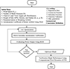 |
Fig. 1 Schematic diagram of morphing blade design. |
2.1 Morphing geometry design method
The reference blade sections are geometrically parameterized to design the MLE and MTE in each blade section. Based on the author’s prior research in reference [29], the proposed morphing parameterization method enables smooth, controlled deflection. The modification is defined by the mean camber line deformation of the airfoils, represented through a polynomial curve. As indicated in Figure 2, the deformation mechanism is represented by an m-degree shape function, expressed as follows: (1)
(1)
 |
Fig. 2 Morphing deformation at the LE and TE. |
In this polynomial, η is the transform value in the y-direction, ξ denotes the non-dimensional length in the x-direction, and is defined within the range 0 ≤ ξ ≤ 1, where ξ = 0 corresponds to the leading edge (LE) and ξ = 1 corresponds to the trailing edge (TE) of the airfoil. α, and β are specified parameters. To satisfy the continuity and smoothness condition at the start and end points of deformation, it should be β = −3 and α = ηLE or α = ηTE, where ηTE and ηLE are the (maximum) deflection values at LE and TE, respectively [30]. Setting m = 2, allows for a second-degree polynomial to be used in generating morphing structures. The second-degree polynomial (m = 2) ensures smooth and controlled morphing deformation while maintaining continuity at transition points (first derivative (slope), and second derivative (curvature) remain continuous across the entire domain, including the leading edge (LE) and trailing edge (TE), satisfying mathematical smoothness conditions). Higher-order polynomials (m ≥ 3) were avoided due to oscillatory behavior (Runge’s phenomenon), numerical sensitivity, undesired inflection points, and increased computational complexity. Previous studies (Ref. [29]) have validated this choice as a practical and efficient method for morphing airfoil applications. The formulations for the Leading Edge (LE) and Trailing edge (TE) transformations are provided as follows:
For the LE transformation: (2)
(2)
For the TE transformation: (3)where x0 is the starting point of the deflection at the leading and trailing edge, and θ is the maximum displacement angle. To obtain the deformed geometry of the LE and TE, the calculated shape function (η) in the y-direction is added to the baseline geometry coordinates. As can be seen in Figure 2, the deformation is restricted to the y-direction, with no changes in thickness distribution and x-coordinates.
The proposed framework offers a computationally efficient and actuator-compatible approach to morphing blade design. Unlike function-based methods such as PARSEC and CST, which redefine the entire airfoil shape, this approach enables localized modifications – a key requirement for real-time actuator control. It ensures smooth and continuous shape transitions, allowing independent control over morphing section locations and deflection angles, making it better suited for aerodynamic adjustments and actuator integration.
A comprehensive optimization process is conducted to determine the optimal deflection angles for the LE and TE (θLE, θTE), their optimal spanwise locations, and the starting points of the deflections ( ). In the results, a negative angle indicates downward motion of the MLE or MTE, while a positive angle indicates upward motion. With three sections along the blade span, this method provides twelve geometric parameters available for optimization. This number reduces to eight if we assume uniform starting points for the MLE and MTE across all blade sections, potentially leading to a simpler morphing mechanism.
2.2 Reference wind turbine
The NREL WindPACT 1.5 MW wind turbine serves as the baseline model for applying the proposed morphing structure and parameterization. This turbine features a 70 m rotor diameter and a 3.5 m hub diameter, resulting in a blade length of 31.5 m, with operation managed through pitch control. As shown in Figure 3, this turbine uses S-series airfoils along its blade span. Additionally, the blade section connected to the hub is circular and gradually transitions into an airfoil shape. The aerodynamic performance characteristics of the wind turbine blade are provided in Table 1. Details of the blade layout distribution are described in reference [31]. The rated wind speed for maximum power output in this turbine is 11.5 m/s, with a corresponding rotor speed of 20.5 rpm. As shown in Figure 4, the blade’s pitch angle dynamically adjusts to maintain constant power output, a factor that must be considered in the morphing blade design across varying wind speeds.
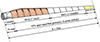 |
Fig. 3 The WindPACT 1.5 MW wind turbine blade. |
2.3 Aerodynamic calculation tools
In morphing blade design, identifying the optimal configurations for the MLE and MTE at different wind speeds is essential, given that the blade operates in dynamic wind environments. Thus, a cost-effective aerodynamic model with sufficient accuracy for fitness evaluation is needed to quantify the performance of each design variable according to predefined objectives. In this study, BEM theory is employed to rapidly evaluate the aerodynamic efficiency of the morphing blade. Following the optimization process, the results are validated through CFD simulations.
2.3.1 BEM method
This study utilizes conventional BEM theory, a widely used method for predicting and optimizing wind turbine performance.
BEM theory is a mathematical model that segments a wind turbine blade into small elements and calculates aerodynamic forces on each element, considering local wind speed, blade geometry, and airfoil characteristics. BEM theory calculates forces on each blade section using airfoil lift and drag coefficients, which are obtained through wind tunnel tests, CFD simulations, or analytical software such as Xfoil/Rfoil. These forces are summed along the blade length to determine the rotor’s overall performance [32]. Several modifications are incorporated into the BEM theory to improve accuracy in predicting wind turbine power extraction and overall performance. First, tip loss and hub loss factors are included to account for the influence of vortices in the generated velocity field. A three-dimensional correction is applied to better simulate the flow field’s three-dimensional behavior. Additionally, Spera’s high-thrust correction model is implemented to address momentum theory inaccuracies in BEM under high-load conditions [33]. Because wind turbine blades often experience high angles of attack beyond the range of 2D wind tunnel data or unconverged Xfoil calculations, it is necessary to extrapolate aerodynamic coefficients for large angles of attack. A common technique is the Viterna approach, which estimates post-stall lift and drag coefficients using a flat-plate assumption [33].
BEM validation with RISO wind turbine
For validation of the BEM code and its modifications, experimental data from the Risø National Laboratory in Denmark were used. The Risø wind turbine has a rated power of 100 kW and features a three-blade rotor with a diameter of 19 m. The turbine reaches maximum power at a wind speed of approximately 14 m/s, with a rotational speed of 47.5 rpm and a pitch angle of 1.8°. Geometric and operational specifications of the Risø wind turbine blade are provided in reference [34]. Experimentally determined aerodynamic coefficients for the airfoils are used in this study [35].
Results from the developed BEM code are compared with Risø wind turbine experimental data in Figure 5. The developed code shows an average error of less than 5% compared to experimental results, demonstrating its suitability for assessing wind turbine power.
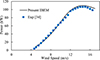 |
Fig. 5 Validation of the BEM method by Risø wind turbine experimental data. |
 |
Fig. 6 Torque and thrust along the blade span of the reference wind turbine at different wind speeds. |
BEM application in baseline WindPACT 1.5 MW wind turbine
Following BEM code validation, the aerodynamic analysis of the WindPACT 1.5 MW wind turbine is conducted in this section. The aerodynamic coefficients of airfoils have been calculated using Xfoil software version 6.99 was used with the e N transition method for boundary layer stability analysis. Simulations were conducted at a Reynolds number of 3.7 × 10⁶, Mach number of 0.14, and Ncrit = 9, representing a free-transition environment suitable for wind turbines with moderate atmospheric turbulence. To ensure convergence, 500 iterations were performed per angle of attack, with 250 panel points enhancing resolution. The angle of attack was varied from −10° to 15° in 0.2° increments, capturing detailed aerodynamic behavior while maintaining computational stability
Figure 6 shows torque and thrust variations along the blade at different wind speeds, with a constant tip speed ratio. It can be seen that the maximum thrust force occurs at 0.9 of the blade length, exerting the greatest influence on rotor torque. Also, doubling the wind speed from 4 to 8 m/s increases maximum torque approximately fourfold, corresponding to a fourfold increase in total thrust force. Since thrust and torque are proportional to the square of wind speed, they increase or decrease accordingly. Discontinuities in the torque and thrust profiles along the blade span result from transitions between different airfoil sections: S818 at the root, S825 at the mid-span, and S826 at the tip.
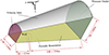 |
Fig. 7 The CFD domain and boundary conditions. |
2.3.2 Computational fluid dynamics (CFD) method
This section outlines the CFD analysis methods used in this study for verification. The incompressible Reynolds-Averaged Navier-Stokes equations are used as governing equations for mass and momentum conservation. The flow field is discretized into finite volume cells to numerically approximate the RANS equations. This study employs the k-ω Shear Stress Transport (SST) model by Menter [36], based on Boussinesq’s hypothesis, to compute turbulence eddy viscosity in the Reynolds stress tensor components. This model resolves turbulence kinetic energy, k, and the specific dissipation rate, ω. The k-ω model is applied in the boundary layer sublayer due to its greater numerical stability over the k-ε model, especially under adverse pressure gradients and compressible flow conditions. Additionally, the model is less sensitive to variations in free-stream ω values. The unsteady continuity and momentum equations, together with the k-ω SST turbulence model, are formulated as: (4)
(4)
![Mathematical equation: $$ \frac{\partial {\bar{u}}_i}{{\partial t}}+\partial {\bar{u}}_j\frac{\partial {\bar{u}}_i}{\partial {x}_j}=-\frac{1}{\rho }\frac{\partial \bar{p}}{\partial {x}_i}+\frac{\partial }{\partial {x}_j}\left[v\left(\enspace \frac{\partial {\bar{u}}_i}{\partial {x}_j}+\enspace \frac{\partial {\bar{u}}_j}{\partial {x}_i}\right)\right]+\frac{\partial }{\partial {x}_j}\left(-\overline{{u}}_i^\mathrm{\prime}{u}_j^\mathrm{\prime}\right);{\tau }_{{ij}}=-\overline{{u}}_i^\mathrm{\prime}{u}_j^\mathrm{\prime};{S}_{{ij}}=\frac{1}{2}\left(\frac{\partial {u}_i}{\partial {x}_j}+\frac{\partial {u}_j}{\partial {x}_i}\right) $$](/articles/stet/full_html/2025/01/stet20240448/stet20240448-eq7.gif) (5)
(5)
 (6)
(6)
 (7)
(7)
In these equations, ρ is the fluid density, ( ) represents the time-averaged velocity component in the ith direction, xi
corresponds to the coordinate in the ith direction, and
) represents the time-averaged velocity component in the ith direction, xi
corresponds to the coordinate in the ith direction, and  denotes the time-averaged pressure. Furthermore, μt
refers to the turbulent viscosity. The constants σk
, σω
, β
*, γ, and β are turbulence model coefficients, and F1 is the blending function between the two formulations of k-ω.
denotes the time-averaged pressure. Furthermore, μt
refers to the turbulent viscosity. The constants σk
, σω
, β
*, γ, and β are turbulence model coefficients, and F1 is the blending function between the two formulations of k-ω.
The k-ω SST turbulence model was selected for its superior accuracy in predicting flow separation, adverse pressure gradients, and boundary layer behavior, which are crucial for morphing airfoils as they alter camber and pressure distribution. Unlike k-ε, it improves near-wall accuracy while maintaining stable free-stream turbulence modeling, making it ideal for wind turbine aerodynamics and validated in previous HAWT studies. Steady-state RANS simulations were used for computational efficiency, while transient simulations (URANS, LES) were excluded but could be explored in future work to assess the blade’s dynamic response.
A pressure-based coupled scheme is used to solve the governing equations. A second-order accurate scheme is employed for discretizing the spatial derivatives. The Single Reference Frame (SRF) method is used to analyze the morphing blade performance. The turbine blade is enclosed within a rotating reference frame that simulates the flow field at the blade’s rotational velocity. The domain inlet conditions include three wind speeds (4, 8, and 11.5 m/s), with a turbulence intensity of 1% based on standard atmospheric boundary layer conditions for offshore sites and a turbulent viscosity ratio of 10 based on ANSYS Fluent User’s Guide. Air pressure and density are set to sea-level conditions.
Figure 7 illustrates the computational domain and boundary conditions. The domain is a frustum-shaped cone with radii of 120 m and 240 m. To reduce computational complexity and mesh size, only a single rotor blade is simulated, as the three blades are symmetrically positioned around the rotational center. The outlet is positioned 350 m (10 rotor radii) downstream of the blade, and the inlet is located 125 m (5 rotor radii) upstream.
 |
Fig. 8 The computational grid around the blade. |
Several grid sizes are used to perform a mesh independence analysis. At a velocity of 6 m/s, the 3D mesh analysis shows a maximum torque deviation of 0.5% between medium and fine grids, leading to the selection of a medium grid with 6.5 million cells for further calculations. Figure 8 depicts the computational grid with unstructured tetrahedral cells. To capture near-wall boundary layer dynamics, a high-resolution mesh with 35 inflation layers is applied to the blade surface. The initial height of the inflated layers is approximately 8.41E-3 mm, calibrated for a non-dimensional wall distance (Y+) close to or below 1. The Y+ value is maintained at this level to accurately capture near-wall flows in turbulent simulations.
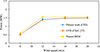 |
Fig. 9 The generated power of the WindPACT 1.5 MW wind turbine at various wind speeds. |
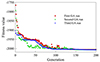 |
Fig. 10 The fitness value against generation number. |
Convergence is achieved when all scaled residuals fall below 10−5. Figure 9 compares generated power at various wind speeds from the current CFD simulations with results from the present BEM method and a referenced numerical study [37]. The figure shows strong agreement between the current CFD results and the CFD calculations from reference [37]. In addition, the present BEM solution produces acceptable results compared to high-fidelity CFD solutions, making it suitable for the iterative optimization process.
2.4 Optimization method
The GA, an optimization technique inspired by natural selection, evolves solutions across generations. Its adaptability, robustness, and global search capabilities make GA ideal for optimizing complex morphing blade designs with numerous design variables, nonlinear behaviors, and multiple objective functions and constraints [38]. These features establish GA as a valuable tool for morphing blade optimization.
This study optimizes geometric variables, including deflection angles at the LE and TE, and the starting points for deformations along each blade section. As shown in Figure 1, these design variables are specified for various operating conditions of a reference wind turbine. The blade comprises three sectional airfoils, each with morphing structures at either the leading or trailing edge. In the most complex configuration, each section includes four design variables (MLE and MTE deflection angles and starting points for both edges), resulting in a total of 12 variables across the three sections. To simplify the morphing mechanism, similar starting points for LE and TE deformations are assumed across all sections, reducing the number of design variables to eight (six deflection angles and two starting points). The deflection angle for the MTE is set between −10° and 4°, while the MLE deflection angle range is −5° to 5°. The starting points for MLE and MTE vary from 0.2 C to 0.35 C and from 0.5 C to 0.9 C, respectively, where C is the chord length of the blade section.
The initial population in GA is generated through random initialization, which assigns values to individuals within specified ranges for each parameter. The GA optimization employs a population size of 20, a maximum of 200 generations, a crossover fraction of 0.6, roulette wheel selection, and a mutation rate of 0.01. Convergence is achieved when either (i) the relative improvement in the best fitness value remains below 10−6 for 50 consecutive generations, or (ii) the algorithm reaches the 200th generation. This dual criterion ensures both computational efficiency and optimal solution stability.
The primary objective of the optimization is to maximize wind turbine power output (kW). To regulate displacements from deflection angles and their lengths, penalty functions (1 and 2) are incorporated into the optimization process. Penalty Function 1 is applied as follows: (8)
(8)
The penalty function constants (A, B, C, D) were selected to ensure balanced contributions from similar morphing parameters and prevent unequal constraints on any single variable. Initial values were estimated based on maximum deflections observed in previous optimizations and refined to assess their influence. The final values kept the penalty function below 4% of the calculated blade power, ensuring structural feasibility and optimization efficiency. For 11.5 m/s, the selected values were A = 28.6, B = 20, C = 0.74, D = 0.32. For 8 m/s, we used A = 20.40, B = 40.0, C = 1.4, D = 0.64, and for 4 m/s, the values were A = 16.5, B = 55.30, C = 2.67, D = 0.87, maintaining consistency across different wind speeds.
An additional analysis was conducted to limit unwanted structural forces on the blades, further restricting excessive movement of the morphing structures, achieved through Penalty Function 2, defined below: (9)
(9)
The constant α is chosen to keep Penalty Function 2 below 4% of the calculated blade power in each generation across all wind speeds. For 11.5 m/s, α = 0.0009, for 8 m/s, α = 0.00052, maintaining a consistent constraint on structural loads, and for 4 m/s, α = 0.0041. The results of applying Penalty Functions 1 and 2 are presented in Section 3.
3 Results and discussion
The morphing blade optimization strategy in this study integrates the GA as the optimizer, BEM theory as the fitness evaluator, and an m-degree shape function for morphing shape parameterization applied to the WindPACT 1.5 MW wind turbine. The optimization process is conducted in three stages: first for the MTE, then for the MLE, and finally for both MLE and MTE simultaneously to maximize power output. The performance of the optimized morphing geometries is then evaluated using CFD analysis.
To verify the optimization results, GA convergence is tracked by plotting fitness values across generations for three independent optimization runs, demonstrating consistent results in finding optimal blade power (Fig. 10). Additionally, Figure 11 tracks variations in four selected parameters across generations to confirm that the algorithm settings effectively explore the search space.
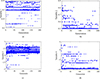 |
Fig. 11 The variations of 4 design variables against generation number. a) Search area of MLE starting point (% C). b) Search area of MTE starting point (% C). c) Search area of MLE angle (°). d) Search area of MTE angle (°). |
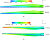 |
Fig. 12 Pressure contours on the surface at rated wind speed. a) Suction side. b) Pressure side. |
3.1 Morphing trailing edge optimization
The morphing blade design begins with a simplified configuration, applying MTEs across different blade sections to evaluate power generation sensitivity and quantify potential power improvements. For this purpose, a minimal set of design variables is used, including the starting point of the MTE deformation (xMTE), varied from 0.5C to 0.9C, and the MTE angles ( ,
,  ,
,  ), varied from +4° to −10° across all three blade sections. The optimization results for MTEs at three wind speeds are presented in Table 2. The findings indicate that the optimization algorithm effectively demonstrates the aerodynamic power benefits of incorporating MTEs across all three blade sections. As wind speed decreases, smaller MTE angles are recommended for the airfoil sections. Power increments of 20.6%, 8.2%, and 7.5% are achieved at wind speeds of 11.5 m/s, 8 m/s, and 4 m/s, respectively. Additionally, the morphed length tends to approach the lower limit of 0.5 C, requiring control constraints to limit this choice.
MTE Optimization results with four design variables.
3.2 Morphing leading edge optimization
In the proposed blade design, the effectiveness of the MLE in enhancing aerodynamic performance is investigated. The initial analysis is conducted with four design variables, as outlined in Table 3, which allow for flexibility in the MLE starting position (xMLE) within the range of 0.2–0.35 C, and the exploration of MLE angles ( ,
,  , and
, and  ) within the range of +5° to −5° for all three airfoils. Results indicate marginal power gains (approximately 0.5%) from this approach, with benefits decreasing as wind speed decreases. Though the objective function shows a minimal increase, annual energy production can still benefit significantly. These cumulative minor improvements could provide meaningful benefits over time, especially when analyzed alongside the regional Weibull distribution curve.
MLE Optimization results with four design variables.
3.3 Simultaneous morphing trailing edge and leading-edge optimization
In this section, the MLE and MTE are optimized simultaneously to create an optimal morphing configuration. Calculations are conducted with 8 design variables per wind speed to maximize power generation using this methodology. Two of these variables represent the starting points of the MLE and MTE deformations along all airfoils (xMTE, xMLE), while three variables represent MLE angles ( ,
,  , and
, and  ), and three variables represent MTE angles (
 ,
,  , and
, and  ) within predefined ranges. The impact of integrating these two morphing structures into the baseline blade – namely MLE and MTE – on aerodynamic power output is presented in Table 4. According to the optimization results, the combination of these features enhances the aerodynamic performance of the wind turbine by approximately 21.7%, 8.69%, and 7.64% at wind speeds of 11.5 m/s, 8 m/s, and 4 m/s, respectively.
Simultaneous MTE and MLE optimization results with eight design variables.
To investigate the maximum potential of the morphing strategy for power generation, optimization is conducted with free deformation lengths on the LE and TE of all three blade sections, increasing the number of design variables from 8 to 12. The results, presented in Table 5, indicate that there is no significant improvement compared to the results obtained with eight variables. Additional analysis examines the impact of the morphing strategy on the thrust force acting on the blade. The data shown in Table 6 reveal a considerable increase in thrust force of up to 62.12% when utilizing the morphing blade. Consequently, alternative objective functions are defined to mitigate the structural impacts associated with the morphing concept. The results of this investigation are discussed in the following section.
Simultaneous MTE and MLE optimization results with 12 design variables.
Optimization results using penalty functions with 8 design variables.
3.4 Optimization with structural constraints
After identifying the optimal deformable blade shapes for each wind speed, as presented in Table 5, the goal of this section is to optimize the morphing blade configuration while ensuring structural feasibility by introducing penalty functions that constrain excessive displacement and thrust force. By applying these constraints, the study aims to maintain high aerodynamic efficiency while reducing actuator energy consumption and preventing mechanical stress on the turbine blade. This need arises due to potential precision variations in decimal values during the GA convergence process, which could lead to significant changes in design variables and increased actuator energy demands. To address this issue, penalty functions (Sect. 2.3) were introduced to constrain design parameters while minimizing power loss. This approach aims to reduce total displacement within the morphing structure. Parameters affecting actuator energy use are defined below by the absolute values of morphing lengths, MLE angles, and MTE angles. (10)
(10)
 (11)
(11)
 (12)
(12)
The thrust force acting on the turbine blade is another key consideration. As shown in Table 5, thrust force can increase by up to 60% with optimal morphing configurations. Therefore, Penalty Function 2 was introduced to limit this force. As shown in Table 6, Penalty Function 1 results in a maximum power reduction of only 0.7%. However, it reduces morphed length by 9.2%, 4.2%, and 13% at wind speeds of 11.5 m/s, 8 m/s, and 4 m/s, respectively. At these wind speeds, total LE angle movement across the three blade sections decreased by 47.5%, 99%, and 99.5%, while total TE angle movement decreased by 1.5%, 21.6%, and 20%. Table 6 also shows that Penalty Function 1 reduces thrust force by 3.5%, 6.82%, and 5% compared to unconstrained optimization at wind speeds of 11.5 m/s, 8 m/s, and 4 m/s, respectively.
Since Penalty Function 1 achieves only minor reductions in thrust force, Penalty Function 2 is applied, with its impact on thrust force control shown in Table 6. Applying this penalty function reduces thrust force by 11.9%, 6.57%, and 6.83% at wind speeds of 11.5 m/s, 8 m/s, and 4 m/s, respectively a more substantial reduction than that achieved with Penalty Function 1. However, this penalty function results in an overall power increase that is 1.6% lower than the increase observed without any penalty functions. With Penalty Function 2, reductions in morphed length of 6.89%, 2.82%, and 9.5% were recorded at these wind speeds. Additionally, total LE angle movement decreased by 10.05%, 14.7%, and 21.3%, while TE angle movement decreased by 9.12%, 18.5%, and 21%, respectively.
3.5 CFD results
This study evaluates optimized morphing blade geometries using CFD simulations. Table 7 presents the calculated power output for these optimized configurations, as detailed in Table 4, across different wind speeds. Power outputs from the baseline and optimized morphing blades are compared using CFD analysis, demonstrating strong agreement with the BEM results in Table 4. At rated wind speed, both CFD and BEM methods estimate significant power gains of 23.8% and 21.7%, respectively, over the baseline blade. Additionally, Table 7 presents CFD results at two other wind speeds (4 m/s and 8 m/s), which align with prior BEM outcomes, showing reduced power gains at non-rated speeds. Figure 12 illustrates pressure contours on the blade surface at rated wind speed, highlighting increased loading as a primary contributor to enhanced turbine power. This additional loading from the morphing blade configuration is observed on both the suction and pressure sides of the blade.
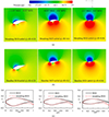 |
Fig. 13 The morphing geometries at three sections and their pressure contours at rated wind speed. a) Morphing blade by MLE and MTE. b) Baseline blade. c) Geometries of the baseline and morphing airfoils. |
Power calculations of morphing blades at different wind speeds by CFD.
Figures 13a and 13b display pressure distributions over the blade sections at 28%, 60%, and 96% of the blade radius under rated conditions. The morphing blade shows improved performance across all sections, with greater pressure differences observed in the middle and tip sections compared to the root. Figure 13c further illustrates the optimal morphing geometries at rated conditions compared to the baseline blade airfoils, highlighting the achieved performance improvements. Figure 14 presents surface pressure coefficients along three blade sections at 0.28, 0.6, and 0.96 of the blade radius. In each section, the morphed blades exhibit a higher leading-edge suction peak compared to the baseline. Additionally, the trailing-edge pressure coefficients are negative in the morphing configuration. Increased lower surface pressure coefficients are observed across all sections compared to the baseline model. The resulting greater pressure difference between the upper and lower surfaces generates increased lift force, subsequently increasing the torque applied to the rotor.
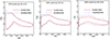 |
Fig. 14 Surface pressure coefficients of blade sections at rated wind speed 11.5 m |
The proposed optimization framework evaluates the effects of morphing leading-edge (MLE) and morphing trailing-edge (MTE) technologies on HAWTs. Results indicate that MTE alone improves power generation by 20.6% at rated wind speed, while MLE, though beneficial, has a less significant independent effect. However, the combined application of MLE and MTE yields the highest performance improvement, with a total increase of 21.7% at rated wind speed. This combination also provides flexible control over structural impacts through the use of appropriate constraint functions. Additionally, the study highlights challenges associated with these technologies, such as the requirement for advanced control systems and the limited effectiveness of MLE when used independently. The selected wind speeds (4 m/s, 8 m/s, and 11.5 m/s) represent key operational points of the 1.5 MW WindPACT turbine, covering low-speed, part-load, and rated conditions. Beyond the rated speed, rotational speed remains fixed, and power is regulated through blade pitch control, keeping morphing behavior aligned with rated conditions.
This study has provided a comprehensive analysis of aerodynamic optimization and morphing blade geometry. However, several important areas remain for future investigation to further enhance the practical application and performance of morphing systems in real-world conditions. These include: the impact of extreme weather conditions, energy consumption of actuators, integration of Fluid-Structure Interaction (FSI) analysis and finally, improving computational models and optimization techniques to dynamically adjust blade configurations using real-time environmental data, allowing for more accurate predictions and more efficient optimization of the morphing process.
4 Conclusions
This study demonstrates the effectiveness of morphing blade technology in enhancing the efficiency of the 1.5 MW NREL WindPACT wind turbine through targeted modifications to the leading and trailing edges. Using a minimal number of design variables, the optimal configurations were identified through a GA-based optimization framework, striking a balance between aerodynamic performance and structural constraints.
Trailing-edge morphing alone yielded a substantial 20.6% power gain at the rated wind speed of 11.5 m/s, while leading-edge morphing provided only marginal independent benefits. However, combining both morphing leading-edge (MLE) and trailing-edge (MTE) technologies resulted in a power increase of 21.7%. The CFD simulations confirming a slightly higher enhancement of 23.8%.
Two penalty functions were introduced to address structural and operational challenges. Penalty Function 1 effectively reduced morphing displacements, with decrease of up to 13% in morphed length and up to 99.5% in leading and trailing-edge angle movements while incurring only a 0.7% reduction in power output. Penalty Function 2 focused on minimizing structural loads, achieving an 11.9% reduction in thrust force with a 1.6% decrease in overall power gain. These constraints make the system viable for practical implementation, as they balance energy efficiency with structural durability and actuator energy requirements.
Moreover, this work highlights the adaptability of morphing blade design across various wind speeds, demonstrating that even minor aerodynamic improvements can significantly increase daily and annual energy production. By integrating advanced objective functions and control systems, this approach offers a scalable solution to improve the energy efficiency of large-scale wind turbines while addressing key practical limitations. While this study effectively optimizes morphing blade configurations using steady-state simulations, it does not consider transient aerodynamic effects, real-time control, or structural deformations, which are crucial for practical implementation and can be addressed in future works.
Data availability statement
All data supporting the findings of this study are included within the article. Detailed descriptions of the analyses and methodologies used are provided, ensuring full transparency and reproducibility.
References
- Farina A, Anctil A (2022) Material consumption and environmental impact of wind turbines in the USA and globally, Resour. Conserv. Recycl. 176, 9, 1–13. [Google Scholar]
- Alagbada SA (2016) 100 MW wind turbine power plant, in: Nahhas AM, Ibhadode AO (eds), Renewable energy: recent advances, IntechOpen, London, UK, pp. 1–17. [Google Scholar]
- Chehouri A, Younes R, Ilinca A, Perron J (2015) Review of performance optimization techniques applied to wind turbines, Applied Energy 142, 1, 361–388. [CrossRef] [Google Scholar]
- Rehman S, Alam MM, Alhems LM, Rafique MM (2018) Horizontal axis wind turbine blade design methodologies for efficiency enhancement: a review, Energies 11, 3, 1–34. [Google Scholar]
- Dimino I, Lecce L, Pecora R (2017) Morphing wing technologies: large commercial aircraft and civil helicopters, in: Ameduri S (ed), Morphing wing technologies, Butterworth-Heinemann, Italy, pp. 491–515. [Google Scholar]
- Aubrun S, Leroy A, Devinant P (2017) A review of wind turbine-oriented active flow control strategies, Exp. Fluids 58, 10, 1–21. [CrossRef] [Google Scholar]
- Manerikar SS, Damkale SR, Havaldar SN, Kulkarni SV, Keskar YA (2021) Horizontal axis wind turbines passive flow control methods: a review, IOP Conf. Ser. Mater. Sci. Eng. 1136, 012022. [CrossRef] [Google Scholar]
- Pechlivanoglou G (2012) Passive and active flow control solutions for wind turbine blades, PhD Thesis, Technical University of Berlin, Berlin, 236 p. [Google Scholar]
- Bai X, Zhan H, Mi B (2023) A new flow control and efficiency enhancement method for horizontal axis wind turbines based on segmented prepositive elliptical wings, Aerospace 10, 9, 1–22. [Google Scholar]
- Bizon N, Tabatabaei NM, Blaabjerg F, Kurt E (2017) Energy harvesting and energy efficiency: technology, methods, and applications, Springer Nature, Switzerland. [CrossRef] [Google Scholar]
- Schaffarczyk AP (2014) Introduction to wind turbine aerodynamics. Green energy and technology, in: Schaffarczyk AP (ed.), Understanding Wind Power Technology: Theory, Deployment and Optimisation, Springer, Berlin, pp. 1–29. [Google Scholar]
- Muiruri PI, Motsamai OS (2017) Fatigue loads mitigation on horizontal axis wind turbines using aerodynamic devices: a survey, J. Eng. Sci. Technol. Rev. 10, 5, 144–152. [CrossRef] [Google Scholar]
- Lachenal X, Daynes S, Weaver PM (2013) Review of morphing concepts and materials for wind turbine blade applications, Wind Energy 16, 2, 283–307. [CrossRef] [Google Scholar]
- Ferede E, Gandhi F (2018) Load alleviation on wind turbines using camber morphing blade tip, in: Wind Energy Symposium, Kissimmee, Florida, 8–12 January, American Institute of Aeronautics and Astronautics, pp. 1–15. [Google Scholar]
- Bartholomay S, Wester TT, Perez-Becker S, Konze S, Menzel C, Hölling M, Spickenheuer A, Peinke J, Nayeri CN, Paschereit OP, Oberleithner K (2021) Pressure-based lift estimation and its application to feedforward load control employing trailing-edge flaps, Wind Energy Sci. 6, 1, 221–245. [CrossRef] [Google Scholar]
- Castillo AD, Jauregui-Correa JC, Herbert F, Castillo-Villar K, Franco JA, Hernandez-Escobedo Q, Perea-Moreno AJ, Alcayde A (2021) The effect of a flexible blade for load alleviation in wind turbines, Energies 14, 16, 1–14. [Google Scholar]
- Nemati M, Jahangirian A (2020) Robust aerodynamic morphing shape optimization for high-lift missions, Aerosp. Sci Technol. 10, 3, 1–10. [Google Scholar]
- Magrini A, Benini E, Ponza R, Wang C, Khodaparast HH, Friswell MI, Landersheim V, Laveuve D, Contell Asins C (2019) Comparison of constrained parameterisation strategies for aerodynamic optimisation of morphing leading edge airfoil, Aerospace 6, 3, 1–14. [Google Scholar]
- Zhang Z, De Gaspari A, Ricci S, Song C, Yang C (2021) Gradient-based aerodynamic optimization of an airfoil with morphing leading and trailing edges, Appl. Sci. 11, 4, 1–25. [Google Scholar]
- Butbul J, Macphee D, Beyene A (2015) The impact of inertial forces on morphing wind turbine blade in vertical axis configuration, Energy Convers. Manage. 91, 1, 54–62. [CrossRef] [Google Scholar]
- Tan J (2017) Simulation of morphing blades for vertical axis wind turbines, Master thesis, Concordia University, 108 p. [Google Scholar]
- Baghdadi M, Elkoush S, Akle B, Elkhoury M (2020) Dynamic shape optimization of a vertical-axis wind turbine via blade morphing technique, Renew. Energy 154, 3, 239–251. [CrossRef] [Google Scholar]
- Alejandro Franco J, Carlos Jauregui J, Carbajal A, Toledano-Ayala M (2017) Shape morphing mechanism for improving wind turbines performance, J. Energy Resour. Technol. 139, 5, 1–13. [CrossRef] [Google Scholar]
- Wang W, Caro S, Bennis F, Salinas Mejia OR (2014) A simplified morphing blade for horizontal axis wind turbines, J. Sol. Energy Eng. 136, 1, 1–8. [Google Scholar]
- Jia L, Hao J, Hall J, Nejadkhaki HK, Wang G, Yan Y, Sun MA (2021) A reinforcement learning based blade twist angle distribution searching method for optimizing wind turbine energy power, Energy 215, 1, 1–12. [Google Scholar]
- Nejadkhaki HK, Sohrabi A, Purandare TP, Battaglia F, Hall JF (2021) A variable twist blade for horizontal axis wind turbines: modeling and analysis, Energy Convers. Manage. 248, 9, 1–13. [Google Scholar]
- Ali AR, Akhter MZ, Omar FK (2021) Performance enhancement of a small-scale wind turbine featuring morphed trailing edge, Sustain. Energy Technol. Assess. 46, 4, 1–12. [Google Scholar]
- Akhter MZ, Ali AR, Jawahar HK, Omar FK, Elnajjar E (2023) Performance enhancement of small-scale wind turbine featuring morphing blades, Energy 278, 5, 1–20. [Google Scholar]
- Najafian A, Jahangirian A (2023) Optimum design of morphing flaps for improving horizontal axis wind turbine performance, Energy Sci. Eng. 11, 7, 2431–2443. [CrossRef] [Google Scholar]
- Mehdi RA, Ostachowicz W, Luczak M (2016) MARE-WINT: new materials and reliability in offshore wind turbine technology, Springer Nature, Switzerland. [Google Scholar]
- Rinker J, Dykes K (2018) WindPACT reference wind turbines, National Renewable Energy Laboratory (NREL), 31 p. [Google Scholar]
- Letcher TM (2017) Wind energy engineering: a handbook for onshore and offshore wind turbines, Joe Hayton, United Kingdom. [Google Scholar]
- Sørensen JD, Sørensen JN (2011) Wind energy systems: optimising design and construction for safe and reliable operation, Woodhead, Oxford, UK. [Google Scholar]
- Schepers JG, van Wingerden MP, van Kuik GEJ, Ockels RLA. 2002. Final report of IEA Annex XVIII: enhanced field rotor aerodynamics database, Energy Research Center of the Netherlands, ECN-C-02-016, February. [Google Scholar]
- Abbott Ira H, Von Doenhoff AE (1959) Theory of wing sections, including a summary of airfoil data, McGraw-Hill Book Company, New York. [MathSciNet] [Google Scholar]
- Menter FR (1994) Two-equation eddy-viscosity turbulence models for engineering applications, AIAA J. 32, 8, 1598–1605. [CrossRef] [Google Scholar]
- Wang L, Quant R, Kolios A (2016) Fluid structure interaction modelling of horizontal-axis wind Turbine blades based on CFD and FEA, J. Wind Eng. Ind. Aerodyn. 158, 11, 11–25. [CrossRef] [Google Scholar]
- Haupt RL, Haupt SE (2004) Practical genetic algorithms, John Wiley & Sons, New Jersey. [Google Scholar]
All Tables
All Figures
|
Fig. 1 Schematic diagram of morphing blade design. |
| In the text | |
|
Fig. 2 Morphing deformation at the LE and TE. |
| In the text | |
|
Fig. 3 The WindPACT 1.5 MW wind turbine blade. |
| In the text | |
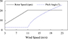 |
Fig. 4 Power control characteristics in the reference WindPACT 1.5 MW turbine [32]. |
| In the text | |
|
Fig. 5 Validation of the BEM method by Risø wind turbine experimental data. |
| In the text | |
|
Fig. 6 Torque and thrust along the blade span of the reference wind turbine at different wind speeds. |
| In the text | |
|
Fig. 7 The CFD domain and boundary conditions. |
| In the text | |
|
Fig. 8 The computational grid around the blade. |
| In the text | |
|
Fig. 9 The generated power of the WindPACT 1.5 MW wind turbine at various wind speeds. |
| In the text | |
|
Fig. 10 The fitness value against generation number. |
| In the text | |
|
Fig. 11 The variations of 4 design variables against generation number. a) Search area of MLE starting point (% C). b) Search area of MTE starting point (% C). c) Search area of MLE angle (°). d) Search area of MTE angle (°). |
| In the text | |
|
Fig. 12 Pressure contours on the surface at rated wind speed. a) Suction side. b) Pressure side. |
| In the text | |
|
Fig. 13 The morphing geometries at three sections and their pressure contours at rated wind speed. a) Morphing blade by MLE and MTE. b) Baseline blade. c) Geometries of the baseline and morphing airfoils. |
| In the text | |
|
Fig. 14 Surface pressure coefficients of blade sections at rated wind speed 11.5 m |
| In the text | |
Current usage metrics show cumulative count of Article Views (full-text article views including HTML views, PDF and ePub downloads, according to the available data) and Abstracts Views on Vision4Press platform.
Data correspond to usage on the plateform after 2015. The current usage metrics is available 48-96 hours after online publication and is updated daily on week days.
Initial download of the metrics may take a while.