")
")
| Issue |
Sci. Tech. Energ. Transition
Volume 80, 2025
Innovative Strategies and Technologies for Sustainable Renewable Energy and Low-Carbon Development
|
|
|---|---|---|
| Article Number | 38 | |
| Number of page(s) | 18 | |
| DOI | https://doi.org/10.2516/stet/2025018 | |
| Published online | 03 June 2025 | |
Regular Article
Research on factors influencing the performance of electric vehicles and its impacts
1
Department of Electrical and Electronics Engineering, Vignan’s Foundation for Science, Technology and Research, Guntur 522213, India
2
Department of Electrical and Electronics Engineering, Indian Institute of Sciences, Bengaluru 560012, India
* Corresponding author: This email address is being protected from spambots. You need JavaScript enabled to view it.
Received:
28
November
2024
Accepted:
2
May
2025
Abstract
Optimizing the forces acting on Electric Vehicles (EVs) is crucial for enhancing performance and energy efficiency, and it is also a key to advancing sustainable transportation. While considerable literature exists on the performance of individual factors, it is felt that there is a gap in the studies that integrate tractive effort, rolling resistance, aerodynamic drag, and hill-climbing force into a unified framework. The present investigation describes a developed comprehensive analytical framework to optimize the combined effects of forces. A systematic analysis is conducted, wherein the work highlights the critical impact of coupling parameters such as tire pressure, road surface, drag coefficient, wind velocity, road grade, vehicle speed, and payload. Some important findings demonstrate that optimal tire pressure and smooth surfaces reduce rolling resistance, while streamlined designs and effective wind management minimize aerodynamic drag, especially at high speeds. Efficient speed and payload management are also essential for maintaining performance on steep inclines. Furthermore, the analysis reveals alignment with FTP-75 driving cycle standards, underscoring accurate performance across parameters, including speed management and energy consumption. It is thought these insights could be helpful to the manufacturers, policymakers, and researchers, emphasizing the importance of considering these coupled relationships in EV design and operation, developing more efficient and sustainable EVs, leading to improved performance, extended range, reduced energy consumption, and enhanced maintenance practices.
Key words: Tractive effort / Rolling resistance power / Aerodynamic drag power / Hill-climbing power / Tire pressure / Road surface / Drag coefficient / Wind velocity / Road grade / Vehicle speed / Payload
© The Author(s), published by EDP Sciences, 2025
 This is an Open Access article distributed under the terms of the Creative Commons Attribution License (https://creativecommons.org/licenses/by/4.0), which permits unrestricted use, distribution, and reproduction in any medium, provided the original work is properly cited.
1 Introduction
The global adoption of Electric Vehicles (EVs) continues to accelerate rapidly, with the available data from Bloomberg NEF (BNEF), EV sales are projected to reach approximately 20% of all passenger vehicle sales worldwide by 2025 [1], highlighting a significant growth trajectory in the automotive market towards electric mobility. Understanding the forces that impact EV performance is crucial for enhancing their efficiency and supporting the transition to sustainable transportation solutions [2, 3]. Key concepts in this study include tractive effort, the force needed to move the vehicle forward; rolling resistance, the frictional force opposing motion due to tire deformation; aerodynamic drag, the resistance experienced as the vehicle moves through the air; hill climbing force, the additional power required to ascend inclines; and acceleration forces, the energy needed to increase speed. For example, according to the Society of Automotive Engineers (SAE) standards, minimizing rolling resistance through advanced tire technologies can significantly extend vehicle range, as seen in Michelin’s low rolling resistance tires [4]. Furthermore, streamlined vehicle designs, such as those used by reputed EV manufacturers, reduce aerodynamic drag and improve energy efficiency, aligning with the International Organization for Standardization (ISO) standards for vehicle aerodynamics [5]. Understanding these forces and their impact on EV performance allows for developing optimization strategies, supporting the transition to greener, more efficient transportation systems.
The literature on tractive effort in electric vehicles highlights the advantages of EVs in terms of energy efficiency and environmental benefits compared to fuel-powered vehicles [6, 7]. The important factors in EV performance modelling include motor torque-speed characteristics, vehicle parameters, and forces acting on the vehicle on various slopes. Among several simulation tools available, MATLAB/Simulink is often used to simulate and optimize these models, helping to predict acceleration and enhance overall performance [8, 9]. A significant aspect impacting vehicle performance is rolling resistance, influenced by road roughness, tyre design, and temperature variations. Minimizing rolling resistance can lead to improved fuel economy, safety, and vehicle handling, making it a critical factor in both vehicle design and road maintenance [10–12]. Moreover, tyre pressure and road surface characteristics are crucial in determining rolling resistance, which directly affects fuel consumption and tyre wear [13–15]. Optimizing tyre pressure and selecting appropriate road surfaces can significantly reduce rolling resistance, enhancing fuel efficiency and tyre longevity [16–18]. Aerodynamic drag is another critical factor impacting vehicle performance. Reducing drag through design innovations and aerodynamic components, such as spoilers and frontal deflectors, can significantly enhance fuel efficiency [19, 20]. Computational Fluid Dynamics (CFD) simulations aid in analyzing aerodynamic forces and optimizing vehicle designs for improved performance [21–23].
Specific factors such as hill climbing force and gradability are essential for various applications, including robotics, military vehicles, and timber harvesting. In EVs and hybrid vehicles, enhancing gradeability and optimizing drivetrain calibration can improve performance on steep inclines [24, 25]. Vehicle mass and acceleration patterns are other crucial factors in energy consumption. Heavier vehicles and varying acceleration rates directly influence fuel efficiency and emissions [26, 27]. In EVs, mass significantly impacts energy consumption in urban driving, while aerodynamic factors are more critical on highways. Implementing energy-efficient control strategies, such as torque vectoring systems, can optimize power distribution and enhance overall efficiency in EVs [28]. Analyzing power consumption across different road conditions, including off-road scenarios, helps in developing strategies to improve EV performance and range, facilitating the broader adoption of electric vehicles [29, 30]. Accurate modelling of tractive forces is vital for predicting driving power and fuel consumption, contributing to energy-efficient control strategies and overall vehicle performance [31]. It is felt that by understanding and addressing these factors, researchers can develop strategies to enhance the efficiency and performance of electric vehicles across different conditions and terrains, supporting their broader adoption and use.
The literature reveals that several gaps exist in the current research on vehicle performance factors. Firstly, studies often analyse performance factors such as rolling resistance, aerodynamic drag, and gradient resistance in isolation rather than in an integrated manner, limiting the understanding of their combined impact on overall EV performance. Additionally, existing research neglects the dynamic nature of tyre pressure variations due to temperature changes and driving conditions. The focus on static aerodynamic features without considering dynamic changes in wind conditions further limits comprehensive analyses. Moreover, the role of road grade in conjunction with other factors like vehicle load and speed is not comprehensively explored. Studies also tend to generalize the effects of payload without accounting for distribution and specific loading conditions. Lastly, there is a notable lack of comprehensive sensitivity analyses examining how variations in key parameters influence overall EV performance. The current investigation attempts to address some of these gaps by developing a comprehensive analytical framework as illustrated in Figure 1. The objective of this work is to optimize the combined effects of various factors influencing EV performance to provide actionable insights for creating more efficient and sustainable EVs. The specific research objectives are:
-
Optimizing the vehicle performance by examining the combined effects of tractive effort, rolling resistance, aerodynamic drag, and hill-climbing force.
- (a)
To quantitatively analyse and demonstrate the impact of tyre pressure variations on the rolling resistance coefficient with respect to vehicle speed.
- (b)
To highlight the importance of road surface quality on rolling resistance power across different road types with respect to vehicle speed.
- (c)
To examine the impact of variable wind velocity conditions & drag coefficient on aerodynamic drag power with respect to vehicle speed.
- (d)
To provide quantitative evidence for supporting the benefits of streamlined vehicle designs by analysing the impact of aerodynamics affecting components like wind velocity and drag coefficient on drag power with respect to vehicle speed.
- (e)
To analyse and understand how road grade influences gradient power requirements with respect to vehicle speed.
- (f)
To emphasize the impact of varying payloads on rolling resistance power and gradient power with respect to vehicle speed.
- (a)
-
To conduct a detailed sensitivity analysis that quantifies the impact of variations in parameters such as tyre pressure, road surface, wind velocity, drag coefficient, road grade, vehicle speed, and payload changes on EV performance.
-
To evaluate EV performance under the Federal Test Procedure 75 (FTP75) drive cycle by assessing speed response, power demands, and overall efficiency during different phases, and to determine compliance with performance standards and practical driving capabilities.
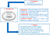 |
Fig. 1 Comprehensive analytical framework for EV performance optimization. |
By achieving these objectives, the research aims to offer a comprehensive understanding of the factors influencing EV performance and contribute to the development of strategies for improving energy efficiency and sustainability in electric vehicle design and operation.
The research work is organized into seven main sections, providing a comprehensive exploration of optimizing electric vehicle performance. Section 1, Introduction: outlines the significance of optimizing EV performance by discussing key concepts, reviewing relevant literature on tractive effort, rolling resistance, aerodynamic drag, and hill-climbing force, identifying gaps in the current research, and presenting the important contribution of the study. Section 2 describes Forces Affecting Vehicle Dynamics, and discusses the key forces affecting vehicle dynamics, including rolling resistance, aerodynamic drag, and gradient resistance, along with detailed algorithms for analysing the forces. It highlights the importance of optimizing factors such as tyre pressure, vehicle speed, road grade, and payload distribution to enhance the efficiency and performance of electric vehicles across various terrains. Section 3, Case Studies, examines the influence of different parameters on EV performance through six cases. Section 4, Performance Analysis of EV under various impacts, presents the sensitivity analysis, and interprets the findings of the research, revealing the sensitivity of the vehicle performance to changes in the input parameters. Section 5, EV under Testing FTP75, outlines the Simulink model for testing an Electric Two-Wheeler with a BLDC motor under the FTP75 drive cycle, focusing on the vehicle’s speed response and performance. Section 6 gives the Results and Discussion wherein analysis of an Electric Two-Wheeler’s performance under the FTP75 drive cycle, covering vehicle speed response, power demands, battery variations, and conformity to FTP75 standards. Finally, Section 7 presents Conclusions: summarizes the key findings, and emphasizes the importance of sensitivity analysis in understanding and optimizing EV performance.
2 Forces affecting vehicle dynamics
The vehicle drive requirements and performance specifications are essential for developing an efficient electric powertrain. Key forces impacting vehicle dynamics include rolling resistance (Frr), aerodynamic drag (Fad), and gradient resistance (Fhc), as illustrated in Figure 2, understanding these forces is crucial for optimizing vehicle performance and energy efficiency.
 |
Fig. 2 Tractive forces impacting vehicle motion. |
The tractive forces involved in propelling a vehicle forward are transmitted to the ground through its drive wheels. Consider a vehicle of mass (m) moving at velocity (v) and ascending a slope at an angle (α) as illustrated in Figure 2, the tractive effort required encompasses various challenges, including:
-
Overcoming the resistance caused by the rolling of its tyres against the road surface.
-
Countering the resistance created by air pressure against the vehicle’s movement.
-
Dealing with the gravitational force pulling the vehicle downhill due to the slope.
-
Providing extra power for acceleration if the vehicle’s speed is not constant.
These tractive forces collectively determine the total force needed to keep the vehicle moving under varying conditions. It is given as [6] (1)
(1)
The total tractive effort power (Pte) required for an electric vehicle to overcome various forces during motion is influenced by multiple components. (2)
(2)
2.1 Rolling resistance power (Prr)
The friction that arises due to the deformation of a tyre as it rolls over the road surface is known as the rolling resistance force, as depicted in Figure 3.
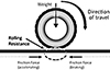 |
Fig. 3 Forces acting on a rolling tire. |
The force acts against the movement of the vehicle, this can be mathematically expressed as (3)
(3)
Rolling resistance power is the power required to overcome the frictional force between the tires and the road surface. It is calculated using the formula: (4)
(4)
Rolling resistance is a linear function of vehicle speed and depends on the coefficient of rolling resistance, which is influenced by the tire material and road surface.
2.1.1 Rolling resistance coefficient analysis
a) The Coefficient as a function of speed for vehicular performance (5)
(5)
This empirical formula can be used for simple vehicle performance calculations. Typically, the coefficient is independent of speed, but it has a very weak relation to vehicle speed as given in equation (5).
b) The rolling resistance coefficient for air-filled tires on dry pavement can be approximated using the following equation [32]: (6)
(6)
Equation (6) is essential in the study for calculating rolling resistance coefficients, crucial for optimizing electric vehicle efficiency based on tire pressure and velocity.
For better understanding and optimizing the rolling resistance, a detailed algorithmic approach is employed. Algorithm 1 calculates the rolling resistance coefficient and rolling resistance power based on variations in tire pressure, rolling resistance coefficient, and vehicle speed.
Require: Arrays of tire pressures (tp) and vehicle speeds (vs)
Ensure: Matrices of rolling resistance coefficients (μrr) and rolling resistance power (Prr)
1. Initialize:
μrr_matrix ← zeros(length(tp), length(vs))
Prr_matrix ← zeros(length(tp), length(vs))
2. Calculate Rolling Resistance Coefficient w.r.t tire pressure variation:
For each tpi in tp
For each vsj in vs
μrr ← Calculate μrr(tpi, vsj); Refer equation (6)

3. Calculate Rolling Resistance Power w.r.t resistance coefficient:
For each μrri in μrr
For each vsj in vs
Prr ← Calculate  ); Refer equation (4)

The rolling resistance coefficient and rolling resistance power calculated through Algorithm 1 provides insights into how variations in tire pressure and vehicle speed impact rolling resistance. This understanding is crucial for optimizing tire maintenance strategies and vehicle design, ensuring better energy efficiency, reducing overall power consumption, and enhancing the performance and lifespan of electric vehicles.
2.1.2 Factors influencing rolling resistance
The coefficient is a function of the weight of the vehicle, tire material and structure, tread geometry, temperature, pressure (as the tire pressure increases its value decreases), road roughness, material, presence and absence of liquids on the road.
Table 1 summarizes coefficients of rolling resistance for various road conditions and surfaces. It highlights different surfaces affect the energy efficiency of vehicles, with lower coefficients indicating smoother surfaces and higher coefficients indicating greater resistance.
Specifications of EV model under testing.
Comparison of EV model under testing.
2.2 Aerodynamic drag power (Pad)
When a vehicle moves through the air at a specific speed, it experiences a force called drag, which opposes its movement. Drag acts in a direction parallel to the airflow.
The air drag is due to two types of driving forces
- (i)
Shape drag: As a vehicle moves forward at a velocity “v”, air impacts the front surface of the vehicle. Not all of this air flows smoothly around and behind the vehicle; some air gets trapped, creating high-pressure zones at the front. Similarly, air flowing towards the rear side of the vehicle does not fill all the voids, leading to low-pressure areas as shown in Figure 4. The difference in pressure between the front and rear of the vehicle generates a force that opposes its motion, known as shape drag. This drag arises because the high-pressure zone pushes the vehicle forward, while the low-pressure area resists its movement.
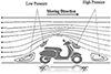
Fig. 4 Aerodynamic forces on a vehicle in motion.
- (ii)
Skin friction: The air in immediate contact with the vehicle’s surface moves at the same speed as the vehicle. However, the air slightly farther away remains nearly stationary. The interaction between these layers of air moving at different speeds creates friction among the air molecules. This frictional force contributes to the overall aerodynamic drag experienced by the vehicle.
The Aerodynamic Drag Force is given by (7)
(7)
Aerodynamic drag power is the power required to overcome the resistance of air as the vehicle moves. It is calculated using the formula: (8)
(8)
Aerodynamic drag power increases exponentially with the vehicle speed, reflecting the cubic relationship between aerodynamic drag and speed.
To optimize and better understand the impact of aerodynamic drag on vehicle performance, a comprehensive algorithmic approach is utilized. Algorithm 2 calculates the aerodynamic drag power based on variations in wind velocity, vehicle speeds, and drag coefficients.
Require: Arrays of wind velocity (vair), vehicle speeds (vs), and drag coefficient (Cd)
Ensure: Matrices of aerodynamic drag power (Pad)
1. Initialize:

2. Calculate Aerodynamic Drag Power w.r.t wind velocity variation:
For each vairi in vair
For each vsj in vs
veff ← vsj + vairi
Pad ← Calculate Pad (ρ, Af, Cd, veff, vsj); Refer equation (8)

3. Calculate Rolling Resistance Power w.r.t drag coefficient:
For each Cdi in Cd
For each vsj in vs
veff ← vsj + vair
Pad ← Calculate Pad (ρ, Af, Cdi, veff, vsj); Refer equation (8)

The aerodynamic drag power is calculated using the Algorithm 2 helps in identifying the variations in drag power with changes in wind velocity and drag coefficient. This understanding is crucial for optimizing the design and performance of electric vehicles, ensuring better energy efficiency and reducing overall power consumption.
2.2.1 Factors influencing aerodynamic drag
Aerodynamic drag is influenced by several factors, including the frontal area and shape of the vehicle, along with protrusions like side mirrors, ducts, and spoilers that disrupt airflow. It also depends on air density, where denser air increases drag, and both the velocity of the vehicle and the relative air velocity play crucial roles, as higher speeds and varying airflow conditions impact the magnitude of drag forces experienced by the vehicle.
The Aerodynamic Drag Coefficient (Cd) is significantly influenced by the design and streamlining of the vehicle. Electric vehicles offer greater flexibility in reducing (Cd) due to the more adaptable placement of components and a diminished necessity for extensive cooling ducts. Additionally, features such as a tapered body, aerodynamic tail cones, the removal of side-view mirrors, lowered ground clearance, and the use of smooth wheel disks contribute to minimizing aerodynamic drag.
Table 2 summarizes the drag coefficients (Cd) and frontal area (Af) ranges for various vehicle types, providing insight into their aerodynamic characteristics.
2.3 Hill climbing power (Phc)
Hill climbing force or gradient resistance occurs when a vehicle travels on an incline. As shown in Figure 5, it is a component of the vehicle’s weight acting along the slope of the incline and is proportional to the sine of the angle (α) of the slope.
 |
Fig. 5 Hilly terrain vehicle movement. |
The hill-climbing force is given by (9)
(9)
Gradient power is the power needed to overcome the gravitational force when the vehicle is moving on an inclined or declined surface. It is calculated using the formula: (10)
(10)
The gradient power is directly proportional to the vehicle speed and the sine of the road grade angle.
Road grade considerations

Gradient resistance power calculations are essential for understanding the vehicle’s performance on different inclines, which is a critical factor for energy-efficient electric vehicle design. To accurately analyze the impact of road grade and payload on vehicle performance, a detailed algorithmic approach is employed. Algorithm 3 calculates gradient power and power variation in rolling resistance with respect to payload and road grades.
Require: Arrays of road grades (α), vehicle speeds (vs), and payloads (Pload)
Ensure: Matrices of gradient power (Phc) and rolling resistance power (Prr)
1. Initialize:

2. Calculate Gradient Power w.r.t road grades:
For each αi in α
For each vsj in vs
Phc ← Calculate Phc (m, g, vsj, αi); Refer equation (10)

3. Calculate Power variation in rolling resistance and gradient w.r.t payload:
For each Ploadi in Pload
For each vsj in vs
meff ← m + Ploadi
Phc ← Calculate Phc (meff, g, vsj, α); Refer equation (10)
Prr ← Calculate Prr (μrr, vsj, meff, g, α); Refer equation (4)

The gradient power and rolling resistance power calculated through Algorithm 3 are crucial for understanding the impact of road grades and payload on vehicle performance. This analysis helps in optimizing the design and operational parameters of electric vehicles to ensure they can efficiently handle varying loads and terrains, contributing to enhanced energy efficiency and overall performance.
2.3.1 Factors influencing gradient forces
Gradient forces, essential for hill climbing in electric vehicles, are influenced by factors such as vehicle mass, road grade steepness, gravitational acceleration, vehicle speed, road surface conditions (including uneven surfaces), tire characteristics, payload distribution, and aerodynamic drag. Optimizing these variables is crucial for efficient energy utilization and enhancing overall performance, particularly in the case of uneven surfaces where varying road conditions pose additional challenges. By addressing these factors comprehensively, vehicle design and operational strategies can be fine-tuned to maximize traction and efficiency, ensuring safe and effective performance across diverse terrains.
3 Case studies
Vehicle performance is influenced by numerous factors that affect efficiency, power consumption, and handling. This section explores six cases to understand these influences better. The first case study examines how tire pressure variations impact the rolling resistance coefficient using Algorithm 1, providing insights into optimal tire maintenance. The second study builds on this by analyzing the relationship between the rolling resistance coefficient and the power required to overcome it, using Algorithm 1. The third and fourth studies focus on aerodynamic drag, investigating how wind velocity and aerodynamic drag coefficient variations affect the power needed to counteract drag forces, using Algorithm 2. The fifth case study explores the impact of road grade on gradient power using Algorithm 3, which is essential for optimizing performance on hilly terrains. Lastly, the sixth study examines how different payloads influence both gradient power and rolling resistance power using Algorithm 3, highlighting the importance of load management. Overall, the analyses offer valuable insights for improving vehicle design, efficiency, and performance.
The data provided in Table 3 is utilized for analyzing the forces and power requirements for a vehicle under various conditions, as detailed in Algorithms 1–3 implemented using MATLAB software.
3.1 Case 1: Variation of rolling resistance coefficient with respect to tyre pressure
To optimize the rolling resistance coefficient for the electric vehicle, it is essential to maintain the tire pressure, which is approximately 2.28 bars recommended by manufacturers [33]. From Figure 6, it is evident, that as the tire pressure increases, the rolling resistance coefficient decreases across different vehicle speeds. For instance, at lower pressures (1 bar), the rolling resistance is significantly higher compared to pressures of 2.5 bars and above. Given that 2.28 bars are close to the 2.5 bar curve, maintaining the tire pressure slightly above the recommended level (while staying within safety limits) can minimize the rolling resistance. This reduction in rolling resistance will enhance the vehicle’s overall efficiency, leading to better energy conservation and improved battery performance, especially at higher speeds. For example, at 70 km/h, the rolling resistance coefficient is about 0.021 for 1 bar pressure and approximately 0.009 for 3.5 bar pressure. The inverse relationship underscores the benefits of higher tire pressure in reducing rolling resistance and thereby enhancing vehicle efficiency. Thus, consistently checking and maintaining tire pressure near the optimal range can significantly impact the vehicle’s efficiency, safety, and handling.
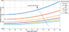 |
Fig. 6 Effect of vehicle speed and tyre pressure on rolling resistance coefficient. |
3.2 Case 2: Impact of rolling resistance power with respect to the rolling resistance coefficient
The analysis of rolling resistance power (Prr) in Figure 7 reveals that optimizing the performance of the vehicle involves carefully selecting road types and managing vehicle speed. The rolling resistance power significantly increases with higher rolling resistance coefficients (μrr), with fields (μrr = 0.30) exhibiting the highest power consumption and surfaces like the wheel on the iron rail (μrr = 0.002) the lowest. For optimal efficiency, it is advisable to drive on roads with lower (μrr = 0.30), such as concrete (μrr = 0.01) and tarmac (μrr = 0.025), and avoid surfaces like loose sand and fields. As vehicle speed increases, rolling resistance power also increases, particularly on high (μrr) surfaces. For instance, driving at 50 km/h on a concrete road results in a rolling resistance power of approximately 1.5 kW, while the same speed on fields results in a much higher 10 kW. Therefore, maintaining moderate speed, especially on surfaces with higher (μrr), is crucial for reducing energy consumption and extending the vehicle’s range. The arrow in Figure 8, indicates “Increasing μrr” emphasizing that higher μrr values lead to higher rolling resistance power, highlighting the critical role of road surface characteristics in energy consumption. Understanding these dynamics is essential for optimizing energy efficiency in electric vehicles through informed route planning, vehicle design, and maintenance strategies.
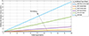 |
Fig. 7 Effect of vehicle speed on resistance power across different road surfaces. |
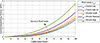 |
Fig. 8 Effect of wind velocity on aerodynamic drag power at different vehicle speeds. |
3.3 Case 3: Variation of aerodynamic drag power with respect to the wind velocity
Figure 8 demonstrates the non-linear increase in aerodynamic drag power (kW) with rising vehicle speeds (0–100 km/h) across various wind velocities. For calm air (0 km/h), drag power climbs from 0 kW to approximately 3.8 kW at 100 km/hr. With light air (5 km/h), it reaches about 4.1 kW, and with gentle wind (10 km/h), it approaches 4.5 kW. Moderate wind (20 km/h) pushes the drag power to around 5.3 kW, and strong wind (40 km/h) elevates it to nearly 7.2 kW. While the impact of wind velocity on drag power is minimal at lower speeds (10–30 km/h), it becomes significant at higher speeds (50–100 km/h). The analysis highlights the significant impact of wind conditions on vehicle performance and underscores the importance of aerodynamic efficiency in automotive design, emphasizing the need to consider wind effects for better energy efficiency.
3.4 Case 4: Variation aerodynamic drag power with respect to the aerodynamic drag coefficient
Figure 9 describes the relationship between aerodynamic drag power (kW) and vehicle speed (km/h) for various drag coefficients (Cd), revealing a non-linear increase in drag power as speed rises, with higher Cd values resulting in significantly higher drag power. At lower speeds (up to 30 km/h), aerodynamic drag power remains relatively low but increases sharply as speed exceeds 60 km/h. For example, at 60 km/h, drag power ranges from approximately 1 kW for Cd = 0.26 to around 2.3 kW for Cd = 0.60, and at 100 km/h, it ranges from about 4.3 kW to nearly 9.5 kW for the same Cd values. The Cd value of 0.26 shows the lowest drag power, indicating superior aerodynamic efficiency compared to higher Cd values. This highlights the critical role of a low drag coefficient in enhancing vehicle performance, particularly at higher speeds where aerodynamic drag becomes a dominant factor, thereby demonstrating the importance of aerodynamic design in improving vehicle efficiency.
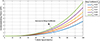 |
Fig. 9 Effect of drag coefficients on aerodynamic drag power across vehicle speeds. |
3.5 Case 5: Variation of gradient power with respect to the road grades
Figure 10 illustrates the linear relationship between gradient power (kW) and vehicle speed (km/h) across various road grades (α), showing that on a flat road (0° grade), no additional gradient power is required regardless of speed. However, as road grades increase, the gradient power needed rises proportionally, with more pronounced demands at higher speeds. For example, at 50 km/h, the gradient power required for a 3° grade is approximately 1.7 kW, increasing to 2.8 kW for a 5° grade. On steeper grades, such as 7° and 11°, the power demands escalate to about 4 kW and 6 kW, respectively, with the steepest grade of 13° requiring around 7.2 kW at the same speed. These insights reveal that higher road grades, combined with increased vehicle speeds, lead to significantly higher gradient power demands. For road grades of 5° and above, these demands increase more sharply, particularly when speeds exceed 25 km/h. To manage gradient power requirements effectively, it is advisable to maintain lower speeds on steeper grades. For instance, keeping speeds below 20 km/h on a 13° grade ensures that gradient power remains under 3 kW, thereby optimizing vehicle performance on challenging inclines and highlighting the necessity for efficient power-train systems in electric vehicles to manage energy consumption across varying road conditions.
 |
Fig. 10 Gradient power vs. vehicle speed for various road grades. |
3.6 Case 6: Variation of gradient power and rolling resistance power with respect to pay loading
Figure 11 presents the correlation between vehicle speed (km/h) and both rolling resistance power (kW) and gradient power (kW) for three different payload percentages: 33.89%, 42.37%, and 50.84%. As the vehicle speed increases, both rolling resistance power and gradient power increase linearly. Higher payload percentages result in greater power requirements at any given speed. For instance, at 100 km/h, the rolling resistance power is approximately 0.33 kW for 33.89% payload, 0.41 kW for 42.37% payload, and 0.48 kW for 50.84% payload. Similarly, the gradient power at 100 km/hr is around 1.18 kW for 33.89% payload, 1.4 kW for 42.37% payload, and 1.7 kW for 50.84% payload. The trend indicates that both rolling resistance and gradient power demands are directly proportional to vehicle speed and payload, with higher payloads significantly elevating power requirements for both metrics.
 |
Fig. 11 Power demand vs. vehicle speed with varying payloads. |
4 Performance analysis of EV under various impacts
This section presents findings from different cases analyzed in Section 3 for various factors affecting vehicle performance. The interpretation of the results is presented in Figure 12 heat map. Figure 12 illustrates the influence of different parameters on performance metrics, highlighting relations and trends. The detailed interpretation of these findings discusses implications and offers insights for optimizing vehicle design and operation through sensitivity analysis.
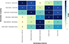 |
Fig. 12 Heat Map of coupling effects on vehicle tractive power components. |
The heat map diagram visually represents the coupling effects of various parameter pairs on key performance metrics of EVs. Each cell in the heat map indicates the strength of the impact that a particular parameter coupling has on a specific performance metric, such as rolling resistance coefficient, rolling resistance power, aerodynamic drag power, gradient power, and tractive power. The scale ranges from 0 (no impact) to 5 (maximum impact), allowing us to see which combinations of parameters are most influential in different performance aspects. When analyzing the coupling effects of different parameters on vehicle performance, it is essential to recognize that these parameters often interact in complex ways. These interactions can either amplify or mitigate the overall impact on performance metrics. The detailed coupling effects of the parameters from the heat map are presented below:
4.1 Tire pressure and road surface
The interaction between tire pressure and road surface condition has a significant impact on the rolling resistance coefficient (μrr) and rolling resistance power (Prr). Based on case 1 analysis, a smooth road surface can help minimize rolling resistance, but if the tire pressure is too low, it can negate the benefits of a smooth surface by increasing the contact area between the tire and the road, leading to higher rolling resistance. Conversely, high tire pressure on a rough surface may reduce the tire’s ability to absorb road irregularities, leading to increased power loss due to vibrations. Thus, maintaining optimal tire pressure is crucial, especially when road surfaces vary. The interaction between tire pressure and the tire of road surface determines the rolling resistance that the vehicle encounters, which directly affects energy efficiency.
4.2 Road surface and road grade
The road surface condition and road grade collectively influence rolling resistance power and gradient power. As described in case 2 and case 5 analysis, the type of road surface coupled with the incline (road grade) critically affects the vehicle’s power requirements. On steep grades, the condition of the road surface can significantly affect the energy required to ascend or descend. A rough surface on an incline increases both rolling resistance and gradient power, leading to higher energy consumption. On a decline, a rough surface can also increase energy requirements due to the need for greater braking force. Managing these parameters together is essential for optimizing energy use and speed management, especially on routes with significant elevation changes.
4.3 Payload changes and road grade
The interaction between payload changes and road grade has a compounding effect on gradient power (Pg) and rolling resistance power (Prr). From the case 6 analysis, it is clear that payload changes, when combined with road grade variations, significantly increase the power required for both gradient and rolling resistance. The heat map results indicate that as the vehicle’s payload increases, the energy required to move the vehicle on an incline also increases proportionally. The impact of this coupling is particularly critical for commercial electric vehicles, which often carry variable loads and operate on routes with varying topography. Managing payload efficiently and adjusting for road grades can lead to substantial energy savings.
4.4 Road grade and vehicle speed
Road grade and vehicle speed are tightly coupled in their effect on gradient power (Pg) and overall energy consumption. This aligns with the case 5 analysis, where higher road grades combined with increased speeds lead to substantial demands on the vehicle’s powertrain. The heat map indicates that as the vehicle speed increases on an incline, the gradient power required also increases, which, in turn, drives up the tractive power needed. This highlights the importance of maintaining lower speeds on steep grades to optimize energy consumption and extend the vehicle’s range.
4.5 Drag coefficient and wind velocity
The drag coefficient (Cd) and wind velocity interact significantly, particularly in influencing aerodynamic drag power (Pad). According to the case 3 analysis, while the drag coefficient determines the baseline aerodynamic drag, wind velocity can either exacerbate or reduce this drag depending on the direction and magnitude of the wind relative to the vehicle’s motion. A higher Cd in strong headwinds will drastically increase drag power, leading to greater energy consumption. While, a lower Cd in tailwinds can reduce drag, improving efficiency. The combination of high Cd and strong wind can be particularly detrimental to vehicle performance, emphasizing the need for aerodynamic optimization, especially in regions with high wind variability.
4.6 Vehicle speed and aerodynamic factors (drag coefficient and wind velocity)
Vehicle speed interacts with aerodynamic factors, particularly drag coefficient and wind velocity, to influence aerodynamic drag power (Pad). As seen in the case 4 analysis, as vehicle speed increases, the influence of the drag coefficient and wind velocity on aerodynamic drag power becomes more significant. For instance, at higher speeds, even slight increases in Cd or adverse wind conditions can lead to a substantial rise in drag power, thereby increasing energy consumption. This coupling suggests that optimizing the vehicle’s shape (to reduce Cd) and operating speed (to minimize adverse wind effects) is crucial for enhancing efficiency, particularly at highway speeds.
From the detailed analysis indicated in Figure 12 heat map, several critical insights into electric vehicle performance optimization emerge. The coupling effects between parameters such as tire pressure, road surface, drag coefficient, wind velocity, road grade, vehicle speed, and payload changes play a critical role in determining overall vehicle performance. These interactions can lead to either compounding effects that increase energy consumption or mitigating effects that enhance efficiency [35, 36]. Understanding and managing these coupled relationships is essential for optimizing electric vehicle design and operation, particularly in practical scenarios wherein multiple factors interact simultaneously. By considering these coupling effects, manufacturers and operators can develop strategies to enhance energy efficiency, reduce operating costs, and improve vehicle performance across diverse conditions.
5 EV under testing FTP75
Evaluating the EV under the FTP-75 driving cycle is crucial to validate the effectiveness of the optimizations derived from the sensitivity analysis. The evaluation not only ensures that the vehicle meets driving standards for energy efficiency but also provides insights into power demand on the motor, battery, and battery energy consumption [37, 38]. Testing these parameters, supports those theoretical improvements that can be translated into practical outcomes essential for assessing practical performance and operational efficiency.
The Simulink model depicted in Figure 13 represents the testing and evaluation of an Electric Two-Wheeler (E2W) driven by a BLDC motor under the FTP75 (Federal Test Procedure 75) drive cycle. The model begins with a drive cycle block providing the speed profile, which is processed by a PID controller to generate the duty cycle and brake signals, with controller parameters set to kp = 0.01, ki = 0.001, and kd = 0.0234. The duty cycle modulates the BLDC motor’s operation, converting electrical energy from the battery into mechanical energy. The battery has a nominal voltage of 72 V, a rated capacity of 56Ah, and starts with a 100% State of Charge (SoC). The motor’s mechanical output is transmitted through the transmission block to the vehicle model, which simulates the vehicle dynamics and outputs the vehicle speed. The model also includes a visualization tool to monitor the vehicle’s speed, ensuring it matches the desired profile. The EV model’s specifications are detailed in Tables 3 and 4, highlighting the vehicle body specifications, and a 5.5 kW motor with a rated speed of 1500 rpm and the battery’s parameters, which influence the vehicle’s performance during the simulation.
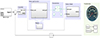 |
Fig. 13 Simulink model of BLDC-driven traction motor for E2W application. |
6 Results and discussion
This section provides a comprehensive analysis of the E2W performance under the FTP75 drive cycle, highlighting its speed response, power demands, and battery behavior. This evaluation is crucial for understanding how the vehicle meets performance standards and handles practical driving conditions. By examining vehicle speed, distance covered, motor and battery power demands, and SoC variations, the analysis offers valuable insights into the efficiency and reliability of the EV, illustrating its ability to perform consistently across different drive phases and ensuring alignment with regulatory standards [39, 40].
6.1 Vehicle response
Figure 14 represents two key aspects of vehicle performance under the FTP75 drive cycle. In Figure 14a, the vehicle’s speed response is shown in relation to time. The red line represents the actual vehicle speed, while the blue line represents the drive cycle source. The drive cycle is divided into distinct phases: Cold Start Transient Phase (lasting 505 s), Stabilized Phase (866 s), Hot Soak Period (628 s), and Warm Start Transient Phase (505 s). During the Cold Start Transient Phase, the vehicle’s speed fluctuates as it adjusts to the drive cycle requirements, covering significant acceleration and deceleration patterns. The Stabilized Phase shows a more consistent speed profile with frequent oscillations, indicating variable driving conditions [41, 42]. The Hot Soak Period represents a period of no vehicle movement, where the speed drops to zero. Finally, the Warm Start Transient Phase shows the vehicle resuming motion, with another series of accelerations and decelerations [43, 44].
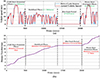 |
Fig. 14 (a) Vehicle speed response and (b) distance travelled by the vehicle under various drive modes. |
Whereas Figure 14b illustrates the distance travelled by the vehicle over the same period. During the Cold Start Transient Phase, the vehicle covers approximately 6 km. In the Stabilized Phase, another 6 km is covered, despite the frequent speed fluctuations. The Hot Soak Period corresponds to no distance travelled, as the vehicle is stationary. The Warm Start Transient Phase resumes distance coverage, with the vehicle covering an additional 5.76 km. The analysis shows how the vehicle’s performance varies across different phases of the drive cycle, with noticeable differences in speed response and distance coverage during transient and stabilized phases [45, 46].
6.2 Power demands
The phase-wise analysis of motor and battery power demands, as shown in Figure 15 aligns closely with the drive cycle phases. During the Cold Start Transient Phase (0–505 s), the motor power demand fluctuates sharply, with peaks up to 15 kW during acceleration and drops to −4 kW during regenerative braking, while the battery power mirrors these fluctuations, peaking at 3.8 kWh and dropping to −4.3 kWh, reflecting effective energy recovery. In the Stabilized Phase (505–1371 s), both motor and battery power demands stabilize, with motor peaks at around 10 kW and battery peaks at 3.65 kWh, indicating steady energy management under consistent driving conditions with variable but smoother speed profiles. The Hot Soak Period (1371–1999 s) shows minimal power activity, with motor and battery power dropping to near zero as the vehicle remains stationary. Finally, during the Warm Start Transient Phase (1999–2504 s), power demands spike again, with motor power reaching up to 15 kW and battery power peaking at 3.8 kWh, along with effective energy recovery during regenerative braking, as the vehicle resumes motion with another series of accelerations and decelerations.
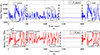 |
Fig. 15 (a) Motor power and (b) battery power demands at various drive modes. |
6.3 Battery SoC and current variations
Figure 16 illustrates the variations in battery SoC and battery current (Ibat) over time during different drive modes. During the Cold Start Transient Phase (0–500 s), the SoC decreases sharply from near 100% to about 94%, indicating a 6% discharge. This decline is due to the high-power demand immediately after the cold start, as reflected by significant fluctuations in battery current, ranging from −400 A to +400 A. The Stabilized Phase (500–1500 s) shows a more gradual decline in SoC, with a 4% discharge, and slightly less intense current fluctuations between −390A and +390A, suggesting that the system has reached a more stable operating condition with lower power demands. The Hot Soak Period (1500–2000 s) is marked by a constant SoC, indicating no discharge, as the battery current stabilizes near zero, confirming minimal or no power draw during this period. Finally, in the Warm Start Transient Phase (2000–2300 s), the SoC experiences another sharp decrease of 4%, similar to the Cold Start Transient Phase, accompanied by significant current fluctuations reaching ±400A, indicating that the battery faces similar transient loads during warm start conditions. Both the Cold Start Transient Phase and Warm Start Transient Phase exhibit sharp SoC decreases due to high current fluctuations and power demands, while the Stabilized Phase shows a more controlled decline with lower power consumption, and the Hot Soak Period indicates no battery utilization.
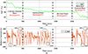 |
Fig. 16 (a) Battery SoC and (b) battery current variation at various drive modes. |
The analysis of Table 5 reveals that the tested EV closely aligns with the FTP-75 driving cycle standards, showcasing its accurate performance across various parameters. The vehicle covers 17.76 km, nearly matching the standard’s 17.77 km and adheres to the duration of 2474 s with minimal variance. Its average speed of 34.09 km/h is also closely aligned with the standard’s 34.12 km/h, indicating consistent speed management. The motor achieves a peak power of 15 kW and generates 62 Nm of torque, demonstrating its capability to handle the drive cycle’s acceleration and deceleration demands, particularly during transient phases. The battery’s peak power of 3.8 kWh and an end-of-test SoC of 85% reflect its effective performance in supporting the motor and managing energy throughout the cycle. Overall, the vehicle’s performance metrics confirm its strong conformity to the FTP-75 standards, highlighting its efficiency and reliability.
7 Conclusion
In the present investigation, an attempt is made to develop a comprehensive analytical framework for optimizing electric vehicle performance by examining the combined effects of tractive effort, rolling resistance, aerodynamic drag, and hill-climbing force under various conditions.
An elaborate sensitivity analysis is conducted and depicted in a heat map, which highlights the strong coupling effects between parameters such as tire pressure, road surface, drag coefficient, wind velocity, road grade, vehicle speed, and payload changes. These interactions significantly influence energy consumption and efficiency, where optimal tire pressure and smooth road surfaces reduce rolling resistance, as described in cases 1 and 2, respectively. Streamlined vehicle designs and wind management minimize aerodynamic drag, particularly at high speeds, which are described in cases 3 and 4.
Furthermore, advanced power-train designs play a crucial role in managing gradient power on steep inclines, efficient vehicle speed, and payload management, which are vital for maintaining performance as described in cases 5 and 6.
The comprehensive analysis presented in Table 5 demonstrates the EV’s close alignment with FTP-75 Driving Cycle Standards, validating its efficiency in speed regulation and energy consumption. It is felt that these insights could offer valuable guidance for manufacturers, policymakers, and researchers, emphasizing the importance of considering these coupled relationships in EV design and operation to develop more efficient and sustainable electric vehicles.
However, the present work is limited to the simulation study and has limitations in considering practical factors such as road irregularities and battery ageing. Hence, future research requires integrating real-time driving data, exploring thermal effects, and conducting experimental validation to refine EV optimization strategies, ultimately enhancing efficiency, range, and overall performance.
References
- Open source: https://about.bnef.com. [Google Scholar]
- Kissai M. (2022) Fundamentals on vehicle and tyre modelling, in: Lenzo B. (ed), Vehicle dynamics. CISM International Centre for Mechanical Sciences, vol. 603, Springer, Cham, pp. 1–59. https://doi.org/10.1007/978-3-030-75884-4_1. [CrossRef] [Google Scholar]
- Gillespie T.D. (2021) Fundamentals of vehicle dynamics, SAE International. ISBN: 1468601768; 9781468601763. [CrossRef] [Google Scholar]
- Wiegand B. (2016) Estimation of the rolling resistance of tires, SAE Technical Paper 2016-01-0445. ISSN:0148-7191. https://doi.org/10.4271/2016-01-0445. [Google Scholar]
- Palin R., Johnston V., Johnson S., D’Hooge A., Duncan B., Gargoloff J. (2012) The aerodynamic development of the Tesla Model S – part 1: overview, SAE Technical Paper 2012-01-0177. ISSN:0148-7191, https://doi.org/10.4271/2012-01-0177. [Google Scholar]
- Hayes J.G., Abas Goodarzi G. (2017) Electric powertrain: energy systems, power electronics and drives for hybrid, electric and fuel cell vehicles. ISBN: 978-1-119-06364-3, https://doi.org/10.1002/9781119063681.ch2. [Google Scholar]
- Naik S.G., Nabi S.M.M. (2024) A comparative analysis of energy consumption in conventional and electric vehicles, Int. J. Veh. Perform. 10, 2, 177–195. https://doi.org/10.1504/IJVP.2024.137691. [CrossRef] [Google Scholar]
- Istiak S.M., Hossain M.R., Tasmin N. (2024) A systematic approach to design electric vehicle powertrains: model-based simulation and real-world application. Int. J. Veh. Perform. 10, 3, 312–348. https://doi.org/10.1504/IJVP.2024.140014. [CrossRef] [Google Scholar]
- Mopidevi S., Dasari K.S., Bakshu S.A., Reddy B.S. (2022) Dynamic performance analysis & sizing of vehicle body & powertrain for 48V electric 2-wheeler system, in 2022 International Conference on Emerging Trends in Engineering and Medical Sciences (ICETEMS), Nagpur, India, 18–19 November, IEEE, pp. 9–14. https://doi.org/10.1109/ICETEMS56252.2022.10093293. [Google Scholar]
- Xu D., Liu X., Shan Y., Gao Q. (2023) Research on impact resistance of steel wheel considering vehicle effect, Int. J. Veh. Perform. 9, 1, 1–15. https://doi.org/10.1504/IJVP.2023.128065. [Google Scholar]
- Wang Y., Shan Y., Xu D., Liu X. (2024) Structural optimisation design of impact resistant composite wheel with compression/injection moulding hybrid structure, Int. J. Veh. Perform. 10, 1, 1–23. https://doi.org/10.1504/IJVP.2024.135449. [Google Scholar]
- Ydrefors L., Hjort M., Kharrazi S., Jerrelind J., Stensson Trigell A. (2021) Rolling resistance and its relation to operating conditions: a literature review, Proc. Inst. Mech. Eng. D: J. Automob. Eng 235, 12, 2931–2948. https://doi.org/10.1177/09544070211011089. [CrossRef] [Google Scholar]
- Levesque W., Bégin-Drolet A., Lépine J. (2023) Effects of pavement characteristics on rolling resistance of heavy vehicles: a literature review, Transp. Res. Rec. 2677, 6, 296–309. https://doi.org/10.1177/03611981221145125. [CrossRef] [Google Scholar]
- Xiuyu L., Al-Qadi I.L. (2022) Integrated vehicle-tire-pavement approach for determining pavement structure-induced rolling resistance under dynamic loading, Transp. Res. Rec. 2676, 5, 398–409. https://doi.org/10.1177/03611981211067797. [Google Scholar]
- Fakhr E.A., Spitas C. (2024) Finite element analysis of studded tyre performance on snow: a study of traction, Veh. Syst. Dyn. 62, 6, 1380–1400. https://doi.org/10.1080/00423114.2023.2232059. [CrossRef] [Google Scholar]
- Kustanto M.N. (2022) The effect of tread pattern tires on hard compound coefficient rolling resistance, J. Mech. Eng. Sci. Innov 2, 2, 55–63. https://doi.org/10.31284/j.jmesi.2022.v2i2.3058. [CrossRef] [Google Scholar]
- Cordoș N., Todoruț A., Iclodean C., Barabás I. (2020) Influence of the dynamic vehicle load on the power losses required to overcoming the rolling resistance, in: Dumitru I., Covaciu D., Racila L., Rosca A. (eds), The 30th SIAR International Congress of Automotive and Transport Engineering. SMAT 2019, Springer, Cham, pp. 195–202. https://doi.org/10.1007/978-3-030-32564-0_23. [CrossRef] [Google Scholar]
- Galati R., Pappalettera A., Mantriota G., Reina G. (2024) Rubber tracks and tyres: a detailed insight into force analysis during obstacle negotiation, Veh. Syst. Dyn. 1–18. https://doi.org/10.1080/00423114.2024.2366528. [Google Scholar]
- Varadarajoo P.K., Ishak I.A., Baharol Maji D.S., Mohd Maruai N., Khalid A., Mohamed N. (2022) Aerodynamic analysis on the effects of frontal deflector on a truck by using Ansys software, Int. J. Integr. Eng. 14, 6, 77–87. https://doi.org/10.30880/ijie.2022.14.06.008. [CrossRef] [Google Scholar]
- Kambiz S., Ortega J.M. (2021) Aerodynamic integration produces a vehicle shape with a negative drag coefficient, Proc. Natl. Acad. Sci. USA 118, 27, 2106406118. https://doi.org/10.1073/PNAS.2106406118. [CrossRef] [Google Scholar]
- Ma X. (2022) Aerodynamic analysis of a car based on computational fluid dynamics and machine learning, in: Proceedings of the ASME 2022 International Mechanical Engineering Congress and Exposition. Volume 8: Fluids Engineering; Heat Transfer and Thermal Engineering, Columbus, Ohio, USA, October 30–November 3, ASME, p. V008T10A010. https://doi.org/10.1115/IMECE2022-96817. [Google Scholar]
- Yuan Z., Xiang W., Zhang H., Zhao Z. (2024) Optimisation study of aerodynamic drag based on flow field topology in box-type trucks, Int. J. Veh. Perform. 10, 1, 96–118. https://doi.org/10.1504/IJVP.2024.135455. [CrossRef] [Google Scholar]
- Munir F.A., Fauzi M.N., Jumaidin R. (2022) Numerical study of the effects of vehicle arrangement on aerodynamics resistance, J. Adv. Res. Fluid Mech. Therm. Sci. 98, 1, 67–72. https://doi.org/10.37934/arfmts.98.1.6772. [CrossRef] [Google Scholar]
- Gerber J.-M., Joubert J.W. (2022) Impact of road grade on the risk profile of driver behavior, Transp. Res. Rec. 2677, 2, 235–245. https://doi.org/10.1177/03611981221089939. [Google Scholar]
- Liu H., Rodgers M.O., Guensler R. (2019) Impact of road grade on vehicle speed-acceleration distribution, emissions and dispersion modeling on freeways, Transp. Res. D: Transp. Environ. 69, 107–122. https://doi.org/10.1016/J.TRD.2019.01.028. [CrossRef] [Google Scholar]
- Kumari S., Ghosh S., Hota A.R., Mukhopadhyay S. (2023) Energy consumption of electric vehicles: effect of lateral dynamics, in: 2023 IEEE 97th (VTC2023-Spring), Florence, Italy, 20–23 June IEEE, pp. 1–5. https://doi.org/10.1109/VTC2023-Spring57618.2023.10200325. [Google Scholar]
- Delaney J.A., McKay B.A., Radcliffe J., Benton D.T., Samozino P., Morin J.B., Duthie G.M. (2022) Uphill sprinting load- and force-velocity profiling: assessment and potential applications, J Sports Sci. 40, 3, 281–287. https://doi.org/10.1080/02640414.2021.1992868. [CrossRef] [PubMed] [Google Scholar]
- Mateichyk V., Soltus A., Klimov E., Kostian N., Smieszek M., Kovbasenko S. (2023) Regularities of changes in the motion resistance of wheeled vehicles along a curvilinear trajectory, Machines 11, 5, 570–570. https://doi.org/10.3390/machines11050570. [CrossRef] [Google Scholar]
- Pardhi S., Deshmukh A., Ajrouche H., Modelling of detailed vehicle dynamics and quantitative impact of electric motor placement on regenerative braking, Int. J. Veh, Perform. 9, 1, 16–40. https://doi.org/10.1504/IJVP.2023.128033. [CrossRef] [Google Scholar]
- Subhani S.C.M., Rao D.V., Vijay Kumar N., GunaSekhar M. (2022) Modeling, aerodynamic and crash simulation on car using fluient, Int. J. Innov. Res. Eng. Manag. 9, 6, 114–118. https://doi.org/10.55524/ijirem.2022.9.6.20. [Google Scholar]
- Widner A., Tihanyi V., Tettamanti T. (2022) Framework for vehicle dynamics model validation, IEEE Access 10, 35422–35436. https://doi.org/10.1109/ACCESS.2022.3157904. [CrossRef] [Google Scholar]
- Open source: https://www.engineeringtoolbox.com. [Google Scholar]
- Open source: https://www.olaelectric.com/s1-pro. [Google Scholar]
- Open source: https://en.wikipedia.org/wiki/FTP-75. [Google Scholar]
- Yalavarthy U.R.S., Kumar N.B., Babu A.R.V., Narasipuram R.P., Padmanaban S. (2025) Digital twin technology in electric and self-navigating vehicles: readiness, convergence, and future directions, Energy Convers. Manage. X 26, 100949. https://doi.org/10.1016/j.ecmx.2025.100949. [Google Scholar]
- Narasipuram R.P., Pasha M.M., Tabassum S., Tandon A.S. (2025) The electric vehicle surge: effective solutions for charging challenges with advanced converter technologies, Energy Eng. 122, 2, 431–469. https://doi.org/10.32604/ee.2025.055134. [CrossRef] [Google Scholar]
- Zhou Z., Wang Y., Zhou G., Liu X., Wu M., Dai K. (2024) Vehicle lateral dynamics-inspired hybrid model using neural network for parameter identification and error characterization, IEEE Trans. Veh. Technol. 73, 11, 16173–16186. https://10.1109/TVT.2024.3416317. [CrossRef] [Google Scholar]
- Chen J., Yu C., Wang Y., Zhou Z., Liu Z. (2024) Hybrid modeling for vehicle lateral dynamics via AGRU with a dual-attention mechanism under limited data, Control Eng. Pract. 151, 106015. https://doi.org/10.1016/j.conengprac.2024.106015. [CrossRef] [Google Scholar]
- Huang Z., Zhou Y., Lin Y., Zhao Y. (2024) Resilience evaluation and enhancing for China’s electric vehicle supply chain in the presence of attacks: a complex network analysis approach, Comput. Ind. Eng. 195, 110416. https://doi.org/10.1016/j.cie.2024.110416. [CrossRef] [Google Scholar]
- Liu K., Jiao S., Nie G., Ma H., Gao B., Sun C., Xin D., Saha T.K., Wu G. (2024) On image transformation for partial discharge source identification in vehicle cable terminals of high-speed trains, High Voltage 9, 5, 1090–1100. https://doi.org/10.1049/hve2.12487. [CrossRef] [Google Scholar]
- Liu Y., Zhao Y. (2024) A blockchain-enabled framework for vehicular data sensing: enhancing information freshness, IEEE Trans. Veh. Technol. 73, 11, 17416–17429. https://10.1109/TVT.2024.3417689. [CrossRef] [Google Scholar]
- Liang J., Yang K., Tan C., Wang J., Yin G. (2025) Enhancing high-speed cruising performance of autonomous vehicles through integrated deep reinforcement learning framework, IEEE Trans. Intell. Transp. Syst. 26, 1, 835–848. https://10.1109/TITS.2024.3488519. [CrossRef] [Google Scholar]
- Zhang J., Hu Y., Li Q., Yin C. (2024) Mechanical performance simulation and optimal design of carbon fiber composite B-pillar, Model. Simul. Mater. Sci. Eng. 32, 6, 065022. https://10.1088/1361-651X/ad6202. [CrossRef] [Google Scholar]
- Fu Y., Dong M., Zhou L., Li C., Yu F.R., Cheng N. (2024) A distributed incentive mechanism to balance demand and communication overhead for multiple federated learning tasks in IoV, IEEE Internet Things J. 12, 10479–10492. https://doi.org/10.1109/JIOT.2024.3510561. [Google Scholar]
- Liu L., Li Z., Kang H., Xiao Y., Sun L., Zhao H., Ma Y. (2025) Review of surrogate model assisted multi-objective design optimization of electrical machines: New opportunities and challenges, Renew. Sustain. Energy Rev. 215, 115609. https://doi.org/10.1016/j.rser.2025.115609. [CrossRef] [Google Scholar]
- Liu X., Tan J., Long S. (2024) Multi-axis fatigue load spectrum editing for automotive components using generalized S-transform, Int. J. Fatigue 188, 108503. https://doi.org/10.1016/j.ijfatigue.2024.108503. [CrossRef] [Google Scholar]
All Tables
All Figures
|
Fig. 1 Comprehensive analytical framework for EV performance optimization. |
| In the text | |
|
Fig. 2 Tractive forces impacting vehicle motion. |
| In the text | |
|
Fig. 3 Forces acting on a rolling tire. |
| In the text | |
|
Fig. 4 Aerodynamic forces on a vehicle in motion. |
| In the text | |
|
Fig. 5 Hilly terrain vehicle movement. |
| In the text | |
|
Fig. 6 Effect of vehicle speed and tyre pressure on rolling resistance coefficient. |
| In the text | |
|
Fig. 7 Effect of vehicle speed on resistance power across different road surfaces. |
| In the text | |
|
Fig. 8 Effect of wind velocity on aerodynamic drag power at different vehicle speeds. |
| In the text | |
|
Fig. 9 Effect of drag coefficients on aerodynamic drag power across vehicle speeds. |
| In the text | |
|
Fig. 10 Gradient power vs. vehicle speed for various road grades. |
| In the text | |
|
Fig. 11 Power demand vs. vehicle speed with varying payloads. |
| In the text | |
|
Fig. 12 Heat Map of coupling effects on vehicle tractive power components. |
| In the text | |
|
Fig. 13 Simulink model of BLDC-driven traction motor for E2W application. |
| In the text | |
|
Fig. 14 (a) Vehicle speed response and (b) distance travelled by the vehicle under various drive modes. |
| In the text | |
|
Fig. 15 (a) Motor power and (b) battery power demands at various drive modes. |
| In the text | |
|
Fig. 16 (a) Battery SoC and (b) battery current variation at various drive modes. |
| In the text | |
Current usage metrics show cumulative count of Article Views (full-text article views including HTML views, PDF and ePub downloads, according to the available data) and Abstracts Views on Vision4Press platform.
Data correspond to usage on the plateform after 2015. The current usage metrics is available 48-96 hours after online publication and is updated daily on week days.
Initial download of the metrics may take a while.