")
")
| Issue |
Sci. Tech. Energ. Transition
Volume 79, 2024
Power Components For Electric Vehicles
|
|
|---|---|---|
| Article Number | 2 | |
| Number of page(s) | 9 | |
| DOI | https://doi.org/10.2516/stet/2023041 | |
| Published online | 09 January 2024 | |
Review Article
Optimal drive cycle current supply of a wound field automotive electrical machine using surrogate models
1
SATIE Laboratory, Stellantis and Paris Saclay University, Carrières-sous-Poissy, France
2
SATIE Laboratory, CY Cergy Paris University, Cergy, France
3
LMSSC, Cnam, HESAM University, Paris, France
4
Stellantis, Carrières-sous-Poissy, France
5
SATIE, Paris Saclay University, Gif-sur-Yvette, France
* Corresponding author: This email address is being protected from spambots. You need JavaScript enabled to view it.
Received:
15
September
2023
Accepted:
15
December
2023
Abstract
Surrogate models have become a widely used solution for reducing computation times along design processes. In this work, a Gaussian Process surrogate model is built and used to predict the performance and losses of a wound field electrical machine in a fast manner. This approach is relevant, especially for drive cycle calculations that rapidly generate rising computation costs if they are computed using physical models, especially finite elements analysis. We present in detail the established method and a comparison of the obtained results with finite elements results. In addition, a detailed analysis of the optimized current supply is presented, and the advantages of variable excitation current are highlighted.
Key words: Drive cycle / Electrical machine / Excitation current / Gaussian process / Metamodeling
© The Author(s), published by EDP Sciences, 2024
 This is an Open Access article distributed under the terms of the Creative Commons Attribution License (https://creativecommons.org/licenses/by/4.0), which permits unrestricted use, distribution, and reproduction in any medium, provided the original work is properly cited.
1 Introduction
Computer experiments i.e., the generation of data by computer codes, are employed in most fields nowadays. In general, computer experiments are deterministic as opposed to real-life experiments where noise and measurement errors can be observed. In optimization problems and many other cases, the computation time of these experiments becomes problematic, leading to the rise of interest in surrogate models.
Surrogate models, also known as metamodels, are constructed using a few sample responses calculated by computer experiments. They are then used to build a surrogate model that is able to give a prediction of the concerned function without additional calls of the computer code [1].
Metamodels have been applied in many fields such as complex physical phenomena approximation [2], groundwater modeling [3], aerodynamic design optimization [4], electrical machine optimization [5], and hybrid electric vehicle optimized control [6]. The application’s framework in this work is electric mobility since hybrid and electric vehicles have gained more and more attention intending to reduce greenhouse gas emissions.
Our focus is on the electrical machine whose optimization is now an inevitable step in the automotive industry. In addition, optimization over the whole drive cycle gives more realistic results than conventional methods that consider only a few operating points. Taking into consideration the whole drive cycle containing thousands of points in the parametric design optimization process is very costly in terms of computation time: based on the numerical tools used in this paper, it can take around 6 years to evaluate 10,000 machines using Finite Elements (FEs). Recent works avoid this problem by presenting drive cycles using a reduced number of operating points in the context of Permanent Magnet Synchronous Machines (PMSMs) optimization [7–10].
In this work, the goal is to develop a fast, versatile, and precise model for current supply optimization that can be integrated into the design optimization process of electrical machines. We present an optimization methodology over the whole Worldwide Harmonised Light Vehicle Test Procedure (WLTP) [11] drive cycle for a Wound Field Synchronous Machine (WFSM) using metamodels.
The choice of sample points and the construction of the surrogate model are detailed. An analysis of the obtained current parameters and the influence of the excitation current are investigated.
Even though this study is focused on electrical machine optimization for automotive applications, the methodology described can be generalized and adapted for predicting other quantities of interest.
2 Electrical machine
Optimization of electric motors is crucial to obtain improved performance and reduced costs. Many types of electric motors are used in the automotive industry [12]. While permanent magnet synchronous machines are dominant, we can also find induction and wound field synchronous motors. The methodology, developed in the following section, is applied to a wound field synchronous machine. The advantages of this type of machine are the absence of permanent magnets and the optimal field weakening operations due to the additional excitation current at the rotor. In fact, WFSMs have three current parameters: armature current density Jind and current angle ψ, as well as the excitation current density Jexc. This third parameter increases the complexity of the problem compared to the case of PMSMs that only have the first two parameters since excitation is fixed by magnets. The 59 kW machine used for the study is taken from [13]. A parametric geometry of the considered e-motor is implemented in MATLAB and interfaced with an external Finite Element Analysis (FEA) software, XFEMM [14]. Figure 1 shows the cross-section of the studied machine, the mesh considered, and flux density for a current density of 10 A/mm2 in both the stator and rotor. Note that mesh size must be carefully chosen since it has a non-negligible impact on computation time. In our case, the FE model is based on a 2D mesh that is composed of 1012 nodes and 1599 triangle elements of order 1 (1599 degrees of freedom). One resolution requires around 5 s1 per operating point (for 15 angular positions). The machine’s meshing has been optimized to ensure that it does not compromise the quality of the quantities of interest (torque, losses, etc.).
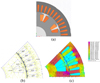 |
Figure 1 Studied WFSM (a) cross-section (b) mesh (c) flux density for 10 A/mm2. |
In this context, the goal is to develop a fast model capable of precise performance evaluation. Many quantities are calculated in a motor such as flux, torque, voltage, and losses. Luckily, not all these quantities need to be predicted using metamodels. Torque and voltage can be analytically calculated using d and q-axes fluxes as in (1) and (2). The dq frame introduced by Park [15] is widely used in electrical machine modeling due to the reduced computation time. Fluxes calculation is initially done in an abc frame considering non-linearity and harmonics. Then, to reduce the complexity the transition to dq frame is done taking into account cross-coupling effects [16]: (1)
(1)
 (2)where
 (3)
(3)
 (4)
(4)
 (5)and
 (6)where Φ
d
, Φ
q
, v
d
, v
q
, i
d
and i
q
are d and q-axes fluxes, voltages, and currents, respectively, p is the number of pole pairs, R is the phase resistance and ψ is the current angle.
(6)where Φ
d
, Φ
q
, v
d
, v
q
, i
d
and i
q
are d and q-axes fluxes, voltages, and currents, respectively, p is the number of pole pairs, R is the phase resistance and ψ is the current angle.
The d and q-axes fluxes are considered independent of the motor speed, so their estimations using metamodels require FE calculations without speed variation. However, this is not the case for iron losses since they cannot be precisely calculated using fluxes for the WFSM [17]. Thus, an additional speed input parameter must be considered in the metamodel building, increasing complexity and computation time. To avoid this, we decided to predict iron losses at two speeds (base and maximum speed). For each speed, a separate metamodel will be created. Since the variation of iron losses as a function of speed can be approximated by a second-order polynomial (Fig. 2), the complexity of the problem can be reduced by fitting a curve using the three-speed points [0, Nbase, Nmax] and the corresponding estimated iron losses at these points [0, ILbase, ILmax]. Note that iron losses are calculated using the method of Bertotti [18].
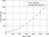 |
Figure 2 Variation of iron losses as a function of speed. |
Figure 3 shows the variation of iron losses at base speed as a function of stator current density and current angle for two different excitation current densities: 5 and 25 A/mm2. We notice that minimum iron losses values are located when excitation and armature current densities have similar values and for maximum current angle (90 degrees). This is where we have maximum flux weakening, d-axis flux being at its minimum and thus giving minimal iron losses values. The same curve trends can also be observed at the maximum speed of rotation of the machine.
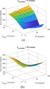 |
Figure 3 Variation of iron losses at base speed. (a) Excitation current density 5 A/mm2; (b) Excitation current density 25 A/mm2. |
Coupling the metamodels with the previous analytical expressions will allow us to compute torque and voltage values. This method is more computationally efficient than FE calculations, where only one computation requires around 15 s of computation time. Considering thousands of operating points and many current input combinations, the finite elements approach is not usable due to the enormous computation times that must be considered.
3 Gaussian process metamodel
Metamodels are built and then used to replace costly classical methods. Two types of metamodels exist: parametric and non-parametric. In the first type, parameters need to be determined for the metamodel construction while in the second, no internal parameter determination is required. Gaussian Process (GP), Radial Basis Functions (RBF), Support Vector Machine (SVM), and Neural Networks (NN) are parametric metamodels, while linear, quadratic, and polynomial regressions are examples of non-parametric metamodels [19].
A GP metamodel is considered in this work [20]. Its distribution is defined by (7), where m is a mean function – generally chosen as a polynomial or as a constant unknown function-, k is a kernel function that models the covariance between each pair in
x
: (7)
(7)
Kernel functions, also known as covariance functions, are a crucial ingredient since they represent the hypothesis we tend to make about the quantity we want to predict. Another critical factor in metamodel creation is the sample points: their number and distribution in space can largely affect the results. These two elements are addressed in detail in the following sections.
3.1 Sample points
Sample points used to build the surrogate model must be carefully chosen to yield good precision along the design space. Many sampling methods exist in the literature [1]. Latin Hypercube Sampling (LHS) has been proven to generate better sample points distribution than random and factorial sampling methods [21], however further improvements can be considered.
Distributed Hypercube Sampling (DHS), interesting for three variables or above, has then been introduced [22]. An additional constraint aims to minimize the coefficient of variation of the minimum distance between sample points projected on 2D surfaces of the hypercube. Compared to classical LHS, DHS adds hypercube surface distributions, but volume distributions are still left out. These distributions are addressed in the improved hypercube sampling IHS [23].
In the following study, sample points are generated based on this IHS method using the multi-DOE toolbox [24]. The number of these points will determine the required computation time and the built metamodel’s prediction accuracy.
3.2 Kernel functions
The kernel function represents the correlation between responses at two points. To better understand this concept, the following example is given. Let x be a sampling point in the design space and y it’s corresponding response and let x ′ be another point in the sampling space that is very close to x . Depending on the studied function, y′ might be close to y in the case of smooth behavior or far if the function presents oscillations. This is where the choice of the kernel function becomes important. Note that in the case of electric machines, a small variation in input current(s) will not usually yield high variation in losses and electromagnetic performances under the same speed and temperature conditions.
Many kernel functions exist and some are more used than others, but one can also build new covariance functions from existing ones [20]. A summary of several commonly used covariance functions is presented in Table 1. A function is called stationary when it is function of
x
–
x
′. In addition, a function is called isotropic if it is a function of r = |
x
–
x′|. The parameter  defines the characteristic length scale and is a constant parameter in the case of isotropic functions while σ corresponds to the standard deviation. These two hyperparameters are optimized using the MATLAB integrated function “fitrgp” [25].
Commonly used covariance functions.
Five of these isotropic functions are chosen for comparison in this study and illustrated in Figure 4: exponential, squared exponential, rational quadratic(α = 1), Matérn 3/2 and Matérn 5/2.
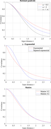 |
Figure 4 Isotropic covariance functions for |

We can create anisotropic versions of these functions by setting  where
M
is a positive semidefinite matrix. In this case, the length scale is no longer constant but varies for each input parameter (i.e. along each component of
x
). Anisotropic versions are also included in the study leading to a total of 10 functions to be compared. The prefix “ard”, corresponding to Automatic Relevance Determinator, is the MATLAB terminology for designating anisotropic functions.
where
M
is a positive semidefinite matrix. In this case, the length scale is no longer constant but varies for each input parameter (i.e. along each component of
x
). Anisotropic versions are also included in the study leading to a total of 10 functions to be compared. The prefix “ard”, corresponding to Automatic Relevance Determinator, is the MATLAB terminology for designating anisotropic functions.
For each of the four quantities to be estimated (ϕ d , ϕ q , ILbase, ILmax), 100 samplings are generated for different sample numbers. This helps us to compare the kernel functions as well as choose the number of sample points needed to obtain the desired accuracy. The Root Mean Squared Error (RMSE) criterion is used to compare these covariance functions. The RMSE is calculated between GP and FE evaluations over 50 independent test points also generated using IHS. The exponential kernel function yields higher mean RMSE for the four quantities of interest, so it is discarded from the comparison.
Figure 5 shows the mean of the RMSE along the 100 considered samplings for each of the four quantities of interest: d and q axes fluxes, iron losses at the base, and maximum speed. The three colors correspond to the different sample point numbers considered (20, 40, and 80) and each point along the x-axis corresponds to one of the four anisotropic kernel functions compared. More detailed graphs can be found in [26] including the four isotropic kernel functions as well as the variance of the RMSE in the comparison. As expected, it is shown that increasing the number of sample points clearly reduces the mean and variance of the errors observed for the four quantities. Nevertheless, the variance has shown very low values compared to the mean of the RMSE. So, unless we want to be very exigent in our choices, we can base our selection of kernel functions on the mean of the RMSE criterion. We also noticed that anisotropic functions yield better results, especially for iron losses estimation. Depending on the application and studied quantities, the kernel function that gives better results may vary.
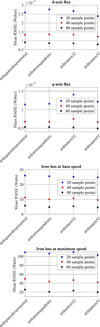 |
Figure 5 Kernel functions comparison for different sample point numbers. |
Depending on the specifications of the studied problem and on the required precision as well as the constraints on computation time, the number of sample points is chosen to respect these previous requirements. For example, if errors greater than 100 W on high-speed iron losses are not tolerated, it is certain that we will need more than 20 sample points to achieve this requirement.
4 Drive cycle application
This section describes the applied drive cycle approach. Forty sample points are used for this study to reduce the needed computation time as much as possible. The kernel function chosen is the anisotropic Matérn 5/2 function for the four quantities of interest. This choice is based on the comparison of kernel functions in the previous section: for 40 sample points, the chosen kernel function is the one that gives the minimum mean RMSE for each of the four quantities.
Once the metamodels are created with the chosen number of sample points and kernel functions conditioning the computation time and precision, we can evaluate fluxes and iron losses for any current inputs in a fast manner. Due to thermal limitations, maximum excitation and current densities are fixed at 15 A/mm2.
Fluxes prediction allows torque and voltage calculations using (1) and (2). Iron losses prediction at two particular speeds is used to create a second-order polynomial. This allows for accurate iron losses estimation for any considered speed as explained in Section 2. Using these predicted quantities along with joule losses, we can create a large table containing these results for different combinations of the three current parameters (Jexc, Jind, ψ). This performance table contains torque, voltage, and losses data for motor mode (0 < ψ <90°) and generator mode (90 < ψ < 180°). The generator mode results are deduced from motor mode results due to symmetry. Since the metamodels give iron losses at two particular speeds, these losses are then adapted for different cycle speeds using polynomial estimation. Using this created performance table, we can search for optimal current inputs allowing us to minimize total losses at each point of the WLTP drive cycle while respecting torque and voltage constraints. Total losses in this case include iron and Joule losses in the stator and rotor. The optimization problem is formulated as follows:
The applied methodology, as well as the computation times associated with each step, are presented in Figure 6 (measured on an Intel® Core ™ i7-10700 CPU @ 2.90 GHz computer with a 32 GB, 2933 MHz RAM). By using the GP models, a few calls to the FE code are required only for building the metamodels, requiring approximately 5 s per call. Then, the four metamodels are created in 60 s. The creation of the performance table along with the adaptation over the drive cycle speeds requires only 5 s, while 35 s are needed for the search for optimal current parameters over the drive cycle.
 |
Figure 6 Flowchart of the drive cycle current optimization method. |
While approximately 5 min are needed to predict the quantities of interest in the performance table using the metamodels (FE calculations of 40 sample points and building the metamodels included), finite element calculations require approximately 30 days to create a performance table of the same size. Thus, one cannot imagine using FE calculations to create the performance table. Repeating this process using only FE models in a design optimization problem of electrical machines will lead to an exorbitant computational cost.
Obtained results from the previously described GP method are compared to FE calculations for identical speed and current inputs. Only the last 800 points of the WLTP drive cycle are presented in Figure 7 to have a closer view of torque and iron losses results. While very good precision is obtained for torque values (mean relative error of 0.1% over the whole drive cycle), iron losses prediction can be improved if more precision is required (mean relative error of 20%). This error is calculated as the average of the relative errors obtained for each operating point of the considered drive cycle as in (8). Reducing the error can be done by increasing the number of sample points: (8)
(8)
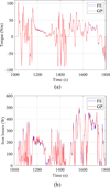 |
Figure 7 Comparison of FE and GP results. (a) Torque; (b) iron losses. |
5 optimal current supply analysis
The previously developed methodology allows optimal current parameter calculations over drive cycles as well as for any point in the speed/torque plane. Current parameters, current angle, losses, and efficiency maps in the speed/torque plane are shown in Figure 8. A maximum torque of 140 Nm and a maximum speed of 12,000 rpm is reached with the used current densities maximum values. For the current angle, we notice an increase, especially for speeds greater than 8000 rpm in order to weaken the d-axis flux and be able to reach these speeds. One can wonder why the flux weakening is obtained by increasing the current angle rather than decreasing the excitation current density. In this section, a detailed explanation and analysis of these results are presented. Thanks to surrogate models, it is possible to analyze the control parameters easily since results are obtained in a fast manner.
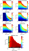 |
Figure 8 Maps obtained for total losses minimization. |
Figure 9 shows torque and total losses values as a function of current angle for different excitation current densities in two cases: Jind = 5 A/mm2 and Jind = 10 A/mm2.
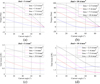 |
Figure 9 Torque and total losses curves for different current inputs. |
For a speed of 10,000 rpm, let us have a closer look at the current parameters needed to achieve a certain torque as well as the resulting losses. Figure 9a shows that obtaining 40 Nm, with a fixed armature current density of 5 A/mm2, requires an excitation current density greater than 7 A/mm2. If we want to achieve flux weakening by reducing this excitation current density, we must increase the level of armature current density to be able to reach the desired torque. For an armature current density of 10 A/mm2, a torque of 40 Nm can be easily achieved by injecting an excitation current density of 5 A/mm2 (Fig. 9b). This will lead to an eventual increase in total losses as can be seen in Figures 9c and 9d. Going from input current parameters [7.5 A/mm2; 5 A/mm2; 21°] to [5 A/mm2; 10 A/mm2; 28°] increases losses by approximately 200 W.
Given that the stator Joule losses are dominant for this machine (refer to the losses maps in Fig. 8) and that the objective of the optimization is to minimize total losses overall operating points, the algorithm will not automatically decrease the excitation current for flux weakening. It will rather find the best combination (Jexc, Jind, ψ) that gives the requested torque while minimizing the total losses.
In order to achieve flux weakening by reducing the excitation current density in this case, we must modify the objective of the optimization to minimize rotor Joule losses rather than minimizing the total losses in the machine. One advantage of this strategy is that losses in the rotor will be reduced, and its thermal management will be easier while extracting calories in the rotor is more difficult to achieve than in the stator. This way, stator Joule losses, and iron losses will not influence the chosen optimal current parameters, and we will observe a decrease in Jexc as the speed increases as shown in Figure 10. As previously discussed, this will lead to an increase in the armature current density to reach the required torque levels. This increase will then affect the stator Joule losses and eventually, the efficiency map shows a noticeable deterioration (Fig. 10) compared to the efficiency map in Figure 8 where all losses are minimized.
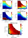 |
Figure 10 Maps obtained for rotor Joule losses minimization. |
The goal of the following paragraph is to study the contribution of a machine with variable excitation compared to a fixed excitation, which is the case of a PMSM, and the influence of this variable excitation on the efficiency in the torque/speed plane.
In order to compare to a PMSM where excitation is fixed by magnets, we can easily fix our excitation current and repeat the same study as above. We notice that for Jexc ≥ 11 A/mm2 we cannot reach all operating points at high speed due to the voltage limitation. On the other hand, for Jexc ≤ 10 A/mm2, we can no longer achieve the maximum torque of 140 Nm. This shows the interest and flexibility of having a variable excitation rather than a fixed one. In order to have a closer look at the influence of a fixed excitation, maps are shown in Figure 11 for Jexc = 10 A/mm2. These maps are obtained for a minimization of the total losses in the machine, including the rotor Joule losses. In this case, a maximum torque of 120 Nm can be reached. To reach higher speeds, the current angle must be considerably increased compared to Figure 8. The efficiency map in this case shows a very small area where the efficiency reaches 96% and a reduced area having an efficiency greater than 94% compared to the efficiency map in Figure 8.
 |
Figure 11 Maps obtained for a fixed excitation current density. |
Figure 12 shows the efficiency map without rotor Joule losses consideration. The objective of this illustration is to approach the case of a PMSM, where we neglect permanent magnet losses. The obtained map is similar to that of an optimized PMSM presented in [27].
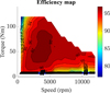 |
Figure 12 Efficiency map relative to a PMSM. |
While the efficiency map relative to a PMSM shows a bigger 97% efficiency area in the middle of the speed/torque plane, the efficiency map of the WFSM (Fig. 8) presents better values at higher speeds.
6 Conclusion
In this work, we developed a Gaussian Process surrogate model to efficiently replace the finite element model of a wound field synchronous machine in order to estimate losses over a drive cycle. Due to the gain in computation time, drive cycle calculations become computationally affordable. The method was described in detail and the associated computation times were presented. A total of 5 min is proved to be sufficient for drive cycle current parameters optimization using the proposed method. It is shown that the most time-consuming step remains the calculation of actual responses at sample points using finite elements analysis. However, the number of calls to the finite elements code is considerably reduced compared to an approach without metamodels.
Enhancing the accuracy of this method can be done by increasing the number of sample points. To further improve precision without increasing the number of sample points, adaptive sampling methods can be proposed [28, 29]. Another area of improvement is to consider a multivariate GP model [30]. This method consists of creating one model with many outputs considering non-separable covariance structures since these outputs are related and modeling them independently might result in the loss of information.
The developed methodology is applied to a predefined wound field synchronous machine topology but is not restricted to this type of motor. It can be exploited in a theoretical manner as in Section 5 to study current parameters and their influence on the energetic performance of the machine. It can also be used in a practical way to determine optimal current inputs of the machine in real-time once the developed model is implemented in a target (Digital Signal Processor (DSP) or Field Programmable Gate Arrays (FPGA) for example). Since no prototype was available, a theoretical analysis is presented and the impact of a variable excitation current is observed, especially for high-speed efficiency, compared to the case of a fixed excitation in PMSM machines.
Given the reduced time costs fulfilled by the metamodel approach, parametric design optimization of electrical machines over a drive cycle will be part of our future work. Since time dependency is no longer eliminated, it will be possible to consider transient phenomena (thermal, electrical, battery charge/discharge phenomena, etc.) in future work.
Conflict of interest
Authors declare no conflict of interest.
Funding
This work is supported by the OpenLab Electrical Engineering for Mobility, Stellantis, France. This CIFRE PhD is co-financed by the ANRT Association.
Intel(R) Core(TM) i7-10700 CPU @ 2.90GHz, 32 GB @ 2933 MHz
References
- Keane A., Forrester A., Sobester A. (2008) Engineering Design via Surrogate Modelling: A Practical Guide, John Wiley & Sons. [CrossRef] [Google Scholar]
- Dupuis R. (2019) Surrogate models coupled with machine learning to approximate complex physical phenomena involving aerodynamic and aerothermal simulations, Doctoral Dissertation. [Google Scholar]
- Asher M.J., Croke B.F.W., Jakeman A.J., Peeters L.J.M. (2015) A review of surrogate models and their application to groundwater modeling, Water Resour. Res. 51, 8, 5957–5973. https://doi.org/10.1002/2015WR016967. [CrossRef] [Google Scholar]
- Tao J., Sun G. (2019) Application of deep learning based multi-fidelity surrogate model to robust aerodynamic design optimization, Aerosp. Sci. Technol. 92, 722–737. https://doi.org/10.1016/j.ast.2019.07.002. [CrossRef] [Google Scholar]
- Duchaud J.L., Hlioui S., Louf F., Gabsi M. (2014) Electrical machine optimization using a kriging predictor, in 2014 17th Int Conf. Electr. Mach. Syst. ICEMS 2014, 3476–3481. https://doi.org/10.1109/ICEMS.2014.7014091. [Google Scholar]
- Harris T.P., Nix A.C., Perhinschi M.G., Wayne W.S., Diethorn J.A., Mull A.R. (2021) Implementation of radial basis function artificial neural network into an adaptive equivalent consumption minimization strategy for optimized control of a hybrid electric vehicle, J. Transp. Technol. 11, 4, 471–503. https://doi.org/10.4236/jtts.2021.114031. [Google Scholar]
- Sun X., Shi Z., Cai Y., Lei G., Guo Y., Zhu J. (2020) Driving-cycle-oriented design optimization of a permanent magnet hub motor drive system for a four-wheel-drive electric vehicle, IEEE Trans. Transp. Electrif. 6, 3, 1115–1125. https://doi.org/10.1109/TTE.2020.3009396. [CrossRef] [Google Scholar]
- Salameh M., Brown I.P., Krishnamurthy M. (2019) Fundamental evaluation of data clustering approaches for driving cycle-based machine design optimization, IEEE Trans. Transp. Electrif. 5, 4, 1395–1405. https://doi.org/10.1109/TTE.2019.2950869. [CrossRef] [Google Scholar]
- Fatemi A., Demerdash N.A.O., Nehl T.W., Ionel D.M. (2016) Large-scale design optimization of pm machines over a target operating cycle, IEEE Trans. Ind. Appl. 52, 5, 3772–3782. https://doi.org/10.1109/TIA.2016.2563383. [CrossRef] [Google Scholar]
- Djami M., Hage-Hassan M., Marchand C., Krebs G., Dessante P., Belhaj L.A. (2022) Kriging metamodel for electric machines: A drive cycle approach, in 2022 Int. Conf. Electr. Mach. ICEM 2022, 251–256. https://doi.org/10.1109/ICEM51905.2022.9910946. [CrossRef] [Google Scholar]
- Ciuffo B., Maratta A., Tutuianu M., Anagnostopoulos K., Fontaras G., Pavlovic J., Serra S., Tsiakmakis S., Zacharof N. (2015) Development of the worldwide harmonized test procedure for light-duty vehicles: Pathway for implementation in European Union legislation, Transp. Res. Rec. 2503, 1, 110–118. https://doi.org/10.3141/2503-12. [CrossRef] [Google Scholar]
- De Santiago J., Bernhoff H., Ekergård B., Eriksson S., Ferhatovic S., Waters R., Leijon M. (2011) Electrical motor drivelines in commercial all-electric vehicles: A review, IEEE Trans. Veh. Technol. 61, 2, 475–484. https://doi.org/10.1109/TVT.2011.2177873. [Google Scholar]
- Di Gioia A., Brown I.P., Nie Y., Knippel R., Ludois D.C., Dai J., Hagen S., Alteheld C. (2017) Design and demonstration of a wound field synchronous machine for electric vehicle traction with brushless capacitive field excitation, IEEE Trans. Ind. Appl. 54, 2, 1390–1403. https://doi.org/10.1109/TIA.2017.2784799. [Google Scholar]
- Crozier R., Mueller M. (2016) A new MATLAB and octave interface to a popular magnetics finite element code, in Proc. – 2016 22nd Int. Conf. Electr. Mach. ICEM 2016, 1251–1256. https://doi.org/10.1109/ICELMACH.2016.7732685. [Google Scholar]
- Park R.H. (1929) Two-reaction theory of synchronous machines: generalized method of analysis – part I, Trans. Am. Inst. Electr. Eng. 48, 3, 716–727. https://doi.org/10.1109/T-AIEE.1929.5055275. [CrossRef] [Google Scholar]
- Herold T., Franck D., Lange E., Hameyer K. (2011) Extension of a d-q model of a permanent magnet excited synchronous machine by including saturation, cross-coupling and slotting effects, 2011 IEEE Int Electr. Mach. Drives Conf. IEMDC 2011, 1363–1367. https://doi.org/10.1109/IEMDC.2011.5994804. [CrossRef] [Google Scholar]
- Mazloum R., Hlioui S., Laurent L., Belhadi M., Mermaz-Rollet G., Gabsi M. (2022) Wound field synchronous drive cycle current parameters optimization: A metamodel-based approach, in 2022 Int. Conf. Electr. Mach. ICEM 2022, 199–205. https://doi.org/10.1109/ICEM51905.2022.9910948. [CrossRef] [Google Scholar]
- Bertotti G. (1987) General properties of power losses in soft ferromagnetic materials, IEEE Trans. Magn. 24, 1, 621–630. https://doi.org/10.1109/20.43994. [Google Scholar]
- Jiang P., Zhou Q., Shao X. (2020) Surrogate-model-based design and optimization, Springer Tracts in Mechanical Engineering (STME). [CrossRef] [Google Scholar]
- Rasmussen C.E., Williams C.K.I. (2006) Gaussian Processes for Machine Learning, Vol. 7, 5, MIT Press, Cambridge, MA. [MathSciNet] [Google Scholar]
- Choi Y., Song D., Yoon S., Koo J. (2021) Comparison of factorial and latin hypercube sampling designs for meta-models of building heating and cooling loads, Energies 14, 2. https://doi.org/10.3390/en14020512. [Google Scholar]
- Manteufel R.D. (2001) Distributed hypercube sampling algorithm, in Collect. Tech. Pap. – AIAA/ASME/ASCE/AHS/ASC Struct. Struct. Dyn. Mater. Conf., vol. 5, pp. 3617–3622. https://doi.org/10.2514/6.2001-1673. [Google Scholar]
- Beachkofski B.K., Grandhi R.V. (2002) Improved distributed hypercube sampling, in Collect. Tech. Pap. – AIAA/ASME/ASCE/AHS/ASC Struct. Struct. Dyn. Mater. Conf. 1, April, pp. 580–586. https://doi.org/10.2514/6.2002-1274. [Google Scholar]
- Laurent L. (2019) MultiDOE: sampling technics on MATLAB/OCTAVE (v3.3). Zenodo. https://doi.org/10.5281/zenodo.2677748. [Google Scholar]
- Mathworks (2019), Statistics and Machine Learning Toolbox User’s Guide R2019b. [Google Scholar]
- Mazloum R., Hlioui S., Laurent L., Belhadi M., Mermaz-Rollet G., Gabsi M. (2022) On the use of surrogate models for drive cycle automotive electrical machine design, in 2022 IEEE Int. Conf. Electr. Sci. Technol. Maghreb, Cist., Vol. 4, pp. 1–6. https://doi.org/10.1109/CISTEM55808.2022.10043894. [Google Scholar]
- Cisse K.M., Hlioui S., Belhadi M., Mermaz-Rollet G., Gabsi M., Cheng Y. (2021) Design optimization of multi-layer permanent magnet synchronous machines for electric vehicle applications, Energies 14, 1–21. https://doi.org/10.3390/en14217116. [Google Scholar]
- Fuhg J.N., Fau A., Nackenhorst U. (2021) State-of-the-art and comparative review of adaptive sampling methods for Kriging, Arch. Comput. Methods Eng. 28, 4, 2689–2747. https://doi.org/10.1007/s11831-020-09474-6. [CrossRef] [MathSciNet] [Google Scholar]
- Xu H., Liu L., Zhang M. (2020) Adaptive surrogate model-based optimization framework applied to battery pack design, Mater. Des. 195, 108938. https://doi.org/10.1016/j.matdes.2020.108938. [CrossRef] [Google Scholar]
- Fricker T.E., Oakley J.E., Urban N.M. (2013) Multivariate Gaussian process emulators with nonseparable covariance structures, Technometrics 55, 1, 47–56. https://doi.org/10.1080/00401706.2012.715835. [CrossRef] [MathSciNet] [Google Scholar]
All Tables
All Figures
|
Figure 1 Studied WFSM (a) cross-section (b) mesh (c) flux density for 10 A/mm2. |
| In the text | |
|
Figure 2 Variation of iron losses as a function of speed. |
| In the text | |
|
Figure 3 Variation of iron losses at base speed. (a) Excitation current density 5 A/mm2; (b) Excitation current density 25 A/mm2. |
| In the text | |
|
Figure 4 Isotropic covariance functions for |
| In the text | |
|
Figure 5 Kernel functions comparison for different sample point numbers. |
| In the text | |
|
Figure 6 Flowchart of the drive cycle current optimization method. |
| In the text | |
|
Figure 7 Comparison of FE and GP results. (a) Torque; (b) iron losses. |
| In the text | |
|
Figure 8 Maps obtained for total losses minimization. |
| In the text | |
|
Figure 9 Torque and total losses curves for different current inputs. |
| In the text | |
|
Figure 10 Maps obtained for rotor Joule losses minimization. |
| In the text | |
|
Figure 11 Maps obtained for a fixed excitation current density. |
| In the text | |
|
Figure 12 Efficiency map relative to a PMSM. |
| In the text | |
Current usage metrics show cumulative count of Article Views (full-text article views including HTML views, PDF and ePub downloads, according to the available data) and Abstracts Views on Vision4Press platform.
Data correspond to usage on the plateform after 2015. The current usage metrics is available 48-96 hours after online publication and is updated daily on week days.
Initial download of the metrics may take a while.