")
")
| Issue |
Sci. Tech. Energ. Transition
Volume 81, 2026
|
|
|---|---|---|
| Article Number | 15 | |
| Number of page(s) | 13 | |
| DOI | https://doi.org/10.2516/stet/2026012 | |
| Published online | 1 mai 2026 | |
Regular Article
Combined machine learning approaches to predict the thermal conductivity of liquid mixtures
1
IFP Energies nouvelles, 1 et 4 Avenue de Bois-Préau, 92852 Rueil-Malmaison, France
2
Condensed Matter Physics Laboratory, University of Thessaly, 35100 Lamia, Greece
* Corresponding author: Cette adresse e-mail est protégée contre les robots spammeurs. Vous devez activer le JavaScript pour la visualiser.
Received:
25
July
2025
Accepted:
13
February
2026
Abstract
The application of Machine Learning (ML)-based techniques was explored to create a fully predictive framework for estimating the thermal conductivity of multi-component mixtures containing hydrocarbons and oxygenated compounds. The study followed these steps: (i) three datasets were constructed using experimental thermal conductivity data for both pure compounds and binary mixtures available in the literature, (ii) symbolic regression was then applied to generate mixing rules considering five independent data manipulation strategies, (iii) new Quantitative Structure-Property Relationship (QSPR) models were developed and benchmarked against work previously published in the literature, and then (iv) QSPR models were used to power mixing rules generated with symbolic regression to predict thermal conductivity values of binary mixtures. A mixing rule was then designed to propose a potential extension to multi-component – two or more components – mixtures. Validation of the latter mixing rule powered with QSPR predictions was performed considering a set of ternary and quaternary mixtures. Finally, the approach was applied to predict the thermal conductivity of four jet fuel samples at different temperatures and atmospheric pressures, resulting in a mean absolute error of 2.9%. Performed comparative analysis confirmed that the developed methodology is effective across a wide range of liquid hydrocarbon and oxygenated mixtures.
Key words: Thermal Conductivity / Mixture / Machine Learning / Fuel / Sustainable Aviation Fuel
Publisher note: The Supplementary material was updated on 6 May 2026.
© The Author(s), published by EDP Sciences, 2026
 This is an Open Access article distributed under the terms of the Creative Commons Attribution License (https://creativecommons.org/licenses/by/4.0), which permits unrestricted use, distribution, and reproduction in any medium, provided the original work is properly cited.
1 Introduction
The reduction of Greenhouse Gases (GHG), more specifically carbon dioxide emissions, has attracted many research in recent decades. The development of energy sources derived from biomass as a replacement for fossil resources is considered a promising alternative. In the context of aviation transport, the development and use of Sustainable Aviation Fuels (SAFs) is one of the pathways seriously envisaged for reducing CO2 emissions. Before introducing a new SAF as a commercial product, either in blend with a fossil fuel or as an aviation fuel in its own, one must ensure that the final product meets the current fuel specifications [1]. In aircraft thermal management systems, the fuel itself acts as an internal heat sink, and it is therefore important to anticipate the impact of SAF’s composition on its thermal properties when designing these fuels, making the thermal conductivity (λ) one of the key properties for jet fuels [2, 3].
The prediction of fuels’ properties using Machine Learning (ML) based approaches has early attracted our attention to derive Quantitative Structure-Property Relationship (QSPR), for instance, to estimate the flash point or cetane number [4, 5]. Recently published reviews addressed the prediction of jet fuel properties including the application of ML-based models [6, 7]. Bohem et al. highlighted the scarcity of data when focusing on λ, and the considered mixing rules were taken from works published in the eighties [6]. Numerous methods have been established to predict the thermal conductivity for pure compounds, and Dehlouz et al. reviewed some existing approaches including the use of Equations of State (EoS) and empirical correlations [8]. Hopp et al. proposed a group-contribution method for the thermal conductivity of pure organic substances based on entropy scaling and an EoS [9]. Comparably, Khosharay et al. developed a thermal conductivity model based on a modified Peng Robinson EoS that can be applied to liquid, vapor, and supercritical regions for conventional refrigerants [10]. Alternatively, QSPR models represent another powerful approach that explicitly connects molecular structure and fluid properties. Our group recently focused on the development of QSPR for the prediction of thermal conductivity for hydrocarbons and oxygenates [3].
The prediction of λ values for mixtures presents additional challenges due to complex interactions occurring between different molecular species. Some empirical mixing rules have been developed and employed to estimate the thermal conductivity of mixtures based on individual λ components and mixture compositions. Several well-known mixing rule equations have been proposed throughout the literature [11], including, for instance, one developed by Filippov and Novoselova [12]: (1)with
  = 0.72, Filippov later reported that for mixtures of chemicals
  ranges from 0.5 to 1.0 and for aqueous solutions from 0.3 to 0.7 [12]. Also reported in reference [11], the mixing rule as proposed by Jamieson and Irving [14]:
 (2)with
  >
>  , or the mixing rule developed by McLaughlin [15]:
 (3)where λ12 is a cross-term coefficient fitted for binary mixture sets under specific constant temperatures. Much more complex equations have been proposed, including various thermophysical properties, for instance, critical properties [16]. In equations (1)–(3), xi and λi denote the composition and thermal conductivity of the mixture component
  , respectively. These equations vary in their theoretical foundations, mathematical complexity, and range of applicability. Most of these mixing rules combine the thermal conductivities of pure components with composition-dependent weighting factors and incorporate additional parameters to account for nonideal mixing behavior.
ML-based techniques now find applications in almost every scientific field, either as predictive methods or as a way to help researchers identify new theories [17]. Genetic Programming (GP) [18], and more recently, Symbolic Regression (SR) represent powerful methods that allow building mathematical models from a dataset without prior assumptions about the form of those models [19, 20]. However, the application of SR to infer symbolic mixing rule expressions from experimental datasets remains, to the best of our knowledge, unexplored [21].
In this work, a two-step ML-based procedure is applied to propose a fully predictive approach for estimating the thermal conductivity for multi-component mixtures. First, SR is used to search for new mixing rule expressions for binary mixtures, then, mixing rules are powered with ML-based model predictions, and a mixing rule expression is proposed for multi-component mixtures. The article is organized as follows: after presenting the data collection and methods applied to develop new ML-based models, the relevance and predictive accuracy of models are discussed by performing comparisons with existing approaches. The article ends with some concluding remarks and perspectives.
2 Materials and methods
2.1 Reference data
The application of ML-based techniques to chemical databases allows identifying non-obvious correlations between property values and molecular features, and has become popular to develop models for the prediction of various physicochemical properties [22]. In such works, the collection of reference experimental data, both in quantity as well as in quality, represents one of the keystones for the success in deriving accurate QSPR models. The experimental thermal conductivity values used as support for the ML modeling were collected from various databases such as the CHEMEO [23], KDB [24], NIST [25], DETHERM [26], and DIPPR [27]. The emphasis was placed on mixtures involving hydrocarbons and oxygenated compounds, at atmospheric pressure and for various temperatures. The range of temperatures covers an interval from 200 K to 600 K. A merger of the collected data has been carried out, resulting, after removing duplicates, in a collection (database labeled DB) of 3053 λ values for 181 binary mixtures at different temperatures. Thus, a total of 32 hydrocarbons and 48 oxygenates are represented in our DB database (Tab. 1).
Contents of the database and its data subsets.
A subset of the database (labeled SDB1) was defined, containing binary mixtures for which, at each considered temperature, the λ value of the individual mixture components is known experimentally. SDB1 includes 1453 λ values for 118 binary mixtures at different temperatures, involving 20 hydrocarbons and 31 oxygenates (Tab. 1). The temperatures covered in SDB1 range roughly from 250 K to 350 K. Figure 1 shows the distributions of chemical families in DB and its subset SDB1, with hydrocarbons and oxygenated compounds representing roughly 40% and 60% of the chemicals, respectively, both in DB and SDB1. Hydrocarbons are categorized in chemical subfamilies such as alkanes, alkenes, and aromatics. Alkanes are predominant both in DB (at a level of 61%) and SDB1 (at a level of 76%). Regarding oxygenated compounds, their population is quite similar within DB and SDB1, with in decreasing order of occurrence: alcohols, ethers, esters, ketones, aldehydes, carboxylic acids. The datasets also contain some multifunctional oxygenates, i.e., compounds containing at least two of the aforementioned functional groups. Each data point in SDB1 is characterized by the binary mixture’s thermal conductivity (λmix), temperature  , and six input features: the mass fractions of components 1 and 2 (
 and
and  , respectively), the thermal conductivity values of components 1 and 2 at
  (
( and
and  , respectively), and the reduced temperatures of components 1 and 2 (
 and
and  , respectively), where:
 (4)with
  being the critical temperature of the compound
  .
.
 |
Figure 1 Distributions of hydrocarbons (black) and oxygenated compounds (dark grey) within the databases. Filled bars stand for samples in the DB database, and dashed bars stand for mixtures in the SDB1 dataset. The values above bars indicate the number of compounds in each chemical subfamily. |
To investigate possible significant discrepancies in the chemical space coverage of DB and its subset SDB1, the t-distributed stochastic neighbor embedding (t-SNE) was applied to samples within these two datasets. The Gaussian Learned Histograms of Distances, Angles, and Dihedrals (GauL-HDAD) method was used to generate a vectorized encoding of each mixture [28]. For this purpose, three-dimensional geometries were obtained starting from the SMILES representations of molecular species converted to unoptimized structures, which were then relaxed using the Merck Molecular Force Field (MMFF94s), as implemented in the RDKit Python library [29, 30]. Afterwards, histograms of interatomic distances, bond angles, and dihedral angles of these optimized geometries were generated to finally create the Gaussian mixture models of mixtures’ components. Notably, each molecule is represented by a fixed-size feature vector whose length equals the total number of Gaussian fits across all histograms, i.e., 158 Gaussian fits across 33 Histograms of Distance, Angle, and Dihedral (HDAD). Finally, for each mixture, the fixed-size feature vectors of individuals were weighted according to the individual compositions, then summed up to define representations for the mixtures. Figure 2 shows the projections of binary mixtures within this chemical space formed by t-SNE1, t-SNE2 and t-SNE3. It demonstrates that with simple topological considerations, it is possible to discriminate binary mixtures. Also, Figure 2 indicates that SDB1 mixtures are generally well distributed within the chemical space defined by DB, suggesting that SDB1 is representative of DB.
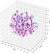 |
Figure 2 Projections of mixture samples into the space formed by t-SNE1, t-SNE2, and t-SNE3. Blue and red symbols stand for mixtures in the DB database and in the SDB1 dataset, respectively. t-SNE1, t-SNE2 and t-SNE3 are unitless. |
A third dataset (SDB2) was built, containing only λ values for pure hydrocarbons and oxygenated compounds for various temperatures. From the DIPPR database [27] only, compounds with more than four experimental λ values at different T were retained, resulting in a total of 1659 data points. To standardize the dataset and ensure uniform representation of compounds, a two-step preprocessing approach was applied as follows: For compounds with more than ten data points, a representative subset of ten points was selected; while for compounds with fewer than ten data points, additional values were generated via interpolation using a second-degree polynomial fit, while remaining in the liquid phase in accordance with literature-reported trends for the temperature dependence of thermal conductivity [3]. Following this procedure, the final SDB2 dataset consists of 1740 experimental and pseudo-experimental data points, with each compound represented by exactly ten data points, maintaining the dataset’s diversity and distribution. More specifically, it resulted in a collection of 66 hydrocarbons and 108 oxygenates (Tab. 1).
2.2 Molecular descriptors
Based on conclusions drawn in previous studies [3–5], Functional Group Count Descriptors (FGCD) derived from the chemical and structural formulae were considered. The FGCD category included counts of atoms and atomic groups identified as chemically relevant. Such a simple representation of compounds has been shown to provide relevant descriptors usable in QSPR modeling. A curated list of FGCD (encoded as SMARTS patterns) was employed to identify and count corresponding substructures within the SMILES representations of compounds in the datasets. The list was constructed in a hierarchical manner, beginning with the most common substructures (e.g., those as proposed by Moreno et al. [3]), followed by class-specific substructures, and finally supplemented with additional patterns to better capture features of compounds that the models struggled to predict accurately. This process was performed sequentially, with the impact of each descriptor on model performance evaluated at each step to decide whether it should be included or not in the final descriptor set. The temperature as well as the molecular weight of each compound were included as additional descriptors,  and
and  , respectively. The complete list of descriptors used is presented in Table 2.
Complete list of descriptors used in the QSPR modeling.
2.3 Machine learning modeling
2.3.1 Mixing rule discovery
The SDB1 database was used as input for searching potential new mixing rule expressions. The GP techniques are interesting methods for performing such an analysis. The basic principle of GP involves randomly setting an initial population of equations and evolving them by applying GP operators mimicking the Darwinian evolution theory of biological species, e.g., selection, crossover, and mutation. During this evolutionary process, each equation is encoded with a tree-like architecture – combinations of variables, mathematical functions, and/or coefficients, as illustrated in Figure 3 – and GP operators act upon sub-tree elements. The population of equations iteratively evolves up to reaching one of the pre-defined criteria such as a best fitness value or the maximum number of iterations (generations). SR is a tool based on these principles, which allows finding suitable mathematical expressions to fit a problem. Among the many codes developed for SR, the PySR (Python Symbolic Regression) library, recently proposed by Cranmer [31], was selected in this work. PySR is highly flexible and allows users to configure various options of the SR process. While some SR settings were left at their default values, others were adjusted according to the problem. Table 3 summarizes investigated values for the population size, the number of iterations, the selected basic mathematical functions for unary and binary operators, and the maximum equation complexity assumed equal to the number of nodes in the tree (e.g., eight in Fig. 3). It is noteworthy that some of the produced trees/equations could be simplified to a lower complexity (e.g., six in Fig. 3). The default loss function (i.e., the mean squared error) was applied.
 |
Figure 3 Illustration of the tree-like architecture representation. X stands for descriptors or variables. |
Adjusted parameter settings for the modeling with PySR.
External validation was performed during the symbolic mixing rule search. The SDB1 dataset was randomly split into Training and Test sets, roughly respecting a ratio of 70:30 (data points). A mixture out strategy was employed [32], ensuring that no mixture present in the Training set appears in the Test set. To enhance the robustness and generalizability of mixing rule models generated by PySR, we adopted five independent data manipulation strategies during the training procedures, as follows:
First, labeled Basic, the Training set was directly utilized without any modifications, aiming to relate thermal conductivity values of data points with the characteristics of the mixture and its components (
 ,
,  ,
,  and
and  ).
).Second, labeled Guided, feature predefinition was achieved by combining the input features (as listed in the previous item) into relevant combinations that reflect known relationships in the thermophysical literature, thus guiding the model toward more physically meaningful expressions.
Third, labeled Shuffling, was introduced to promote symmetry in the resulting expressions with respect to the ordering of components in a binary mixture. We thus implemented random shuffling: the identities of compounds 1 and 2 (and their corresponding features) were randomly interchanged, and model fitting was resumed from the previous fitting state. This shuffling is applied several times during the PySR fitting process so that, by the end, all identities of binary mixture components have undergone transformation.
Fourth, labeled Rearrangement, inspired by equation (2) and related empirical formulations, we introduced a data rearrangement rule where, for each mixture data point, the compound with the higher thermal conductivity value was consistently assigned as compound 1 (i.e., enforcing
 >
>  ).
).Lastly, labeled Augmentation, a data augmentation strategy was employed, where a copy of the Training set was generated with compound identities swapped (i.e., features for compounds 1 and 2 interchanged) and appended to the original Training set. This not only reinforces symmetry but also effectively doubles the training data.
Throughout the SR fitting process, model performance was continuously monitored using PySR’s integrated TensorBoard logger, which provides real-time tracking of both the loss function and the Pareto front volume. This allowed for effective oversight of the trade-off between model complexity and accuracy during the evolutionary process. To ensure the physical validity of the derived expressions, dimensional consistency constraints were enforced, guaranteeing that the resulting equations for thermal conductivity maintained appropriate units.
In addition to modeling the full mixing rule expression, a separate modeling approach was undertaken to isolate and fit only the term expressing the deviation from additivity, considering the additive term as  , a common component in formulations of mixture thermal conductivity, and more generally, such terms are found in other thermophysical properties associated with non-ideal mixing behavior. Modeling this deviation from additivity provides insight into interaction effects between components and supports the construction of more accurate equations. All five aforementioned data manipulation strategies were also applied to modeling only the deviation term.
2.3.2 QSPR modeling
There are multiple ML algorithms that could be employed for performing QSPR modeling. From comparisons in previous studies [4], we demonstrated that using a Support Vector Machine (SVM) with an FGCD-based description of the molecular species generally yields robust QSPR models. In a recent study, we demonstrated that the application of Extreme Gradient Boosting (XGBoost) provides models with performances at least comparable to SVM-based ones [33]. Therefore, both SVM and XGBoost algorithms were applied to the SDB2 dataset to derive QSPR models to predict the thermal conductivity of pure hydrocarbons and oxygenated compounds.
The SVM algorithm attempts to find a hyperplane that linearly separates the data into a high-dimensional feature space, achieved by transforming the original descriptor space through kernel functions. For regression tasks, this approach is adapted into Support Vector Regression (SVR), which constructs a predictive model by minimizing error while controlling model complexity within a predefined tolerance margin. In this work, we employed the Radial Basis Function (RBF) kernel to non-linearly map data into a higher-dimensional space, enabling the model to capture complex relationships between descriptors and λ values. According to this method, up to three hyperparameter values need to be optimized: cost, ϵ, and γ. For this purpose, SVR hyperparameters were optimized in a 5-fold cross-validation procedure, with the parameter space explored accordingly: cost was tested for values between 10 and 300,  values ranged from 4 × 10⁻³ to 1 × 10⁻², and
  values between 2 × 10⁻⁴ and 1 × 10⁻³ were evaluated.
XGBoost is a scalable, ensemble-based ML algorithm that implements gradient boosting, building predictive models by iteratively combining multiple weak learners, typically decision trees. At each iteration, a new tree is trained to correct the residuals of the previous ensemble, optimizing a regularized objective function that balances model fit and complexity. By leveraging gradient information and incorporating techniques such as subsampling, column sampling, and regularization, XGBoost achieves both high predictive accuracy and robustness against overfitting. For our XGBoost-based models, four hyperparameters were optimized: number of boosting rounds (from 50 to 300), maximum tree depth (from 3 to 6), learning rate (from 0.1 to 0.4), and subsample ratio (from 0.5 to 1.0). Other hyperparameters relating to column sampling and regularization were also optimized, but with very little increase to model performance and generalizability hence, these hyperparameters were left at default for the final model.
For both SVR and XGBoost hyperparameters, a Bayesian optimization was performed for 200 iterations, with performance evaluated using 5-fold compound-out – where the ten λ values for a given compound were assigned to the same fold – cross-validation to account for data grouping structure and ensure generalizability. The most optimal hyperparameter configuration was selected based on the highest mean coefficient of determination ( ) score on the external folds.
2.3.3 Performance of models
Models are assessed based on their capacity to predict reference thermal conductivity values. The predicted values are compared to reference experimental data, and the models’ performances are evaluated using specific metrics, such as the Mean Absolute Error (MAE), the Root Mean Squared Error (RMSE), and R2, respectively expressed as follows: (5)
(5)
 (6)
(6)
 (7)
(7)
where  denotes the predicted value,
  the experimental value,
  stands for the average of experimental thermal conductivity values, and N is the number of data points in the considered set. Although MAE and RMSE values retain the unit of the property, the coefficient of determination is unitless. The lower the MAE and RMSE values, the better the predictions; R2 varies between 0 and 1, with values closer to 1 generally indicating better predictive performance.
3 Results and discussion
3.1 New mixing rules discovery
The SDB1 database – containing for each data point experimental λ values for the binary mixture as well as for individual components at the temperature T, mass fractions, and reduced temperatures of components – was used as input for PySR runs to search for new mixing rule expressions. Two approaches consisting of designing a whole equation or only a part, such as the term related to the deviation from additivity, were followed. Also, five independent data manipulation strategies were investigated: Basic, Guided, Shuffling, Rearrangement, and Augmentation. All these PySR runs led to generation of hundreds of mixing rules. Table 4 summarizes the performances of the generated mixing rules when assessed on the SDB1 splitting into Training and Test sets. Only the best performing equation is reported for each approach/strategy and number of iterations. All corresponding equations are reported in the Supplementary material. Additionally, three published mixing rules involving similar variables and widely used in the literature were tested on the same SDB1 subsets.
R 2 and RMSE (in W m−1 K−1) values calculated for the different PySR-generated mixing rules when applied to SDB1 Training and Test sets.
The three mixing rules identified in the literature were used as a reference point for assessing the performance of expressions generated with PySR, and the benchmarking between equation (1) with α = 0.50 or α = 0.72, and equation (2) is proposed in Table 4. The evaluation on the SDB1 Test set for equation (1) with the default constant value (α = 0.72) leads to an R2 value of 0.9736. The same equation used together with the optimised constant value (α = 0.50) yields improved predictions with a R2 value of 0.9764. While predictions using Jamieson and Irving’s model (R2 = 0.9749) outperform those derived from the application of Filippov and Novoselova’s default-constant model, they both remain slightly less accurate to equation (1) with the optimised constant.
Table 4 shows that for the majority of the covered scenarios, generated mixing rules after 105 iterations outperformed or often equaled those resulting from 104 iterations runs, evaluated on the SDB1 Training set. The strategy labeled Augmentation – for which the database size is doubled – seems, however, to necessitate the highest number of iterations to reach a sufficient convergence. In the two strategies labeled Basic and Rearrangement, a marginal decrease is observed in performance with increased training iterations – from 104 to 105 – with, however, a more expected trend when applied to the SDB1 Test set for the Basic strategy. Specifically, the test R2 increases from 0.9766 to 0.9773, and the RMSE shows a slight decrease, supporting the notion of incremental benefits for prolonged optimization. Also, from the results presented in Table 4, it is noteworthy that some of the generated mixing rules consistently match or even outperform equations extracted from the literature. These capabilities emphasize both the robustness and adaptability of our followed modelling approaches.
The approach labeled Whole Equation leads to mixing rules with strong and stable predictive performances roughly across all preprocessing strategies. In every investigated scenario, R2 values calculated on the external SDB1 Test set remain above 0.974, while corresponding RMSE values consistently stayed below 0.0037 W m−1 K−1, indicating excellent generalization capability to unseen binary mixtures. Among all scenarios, the strategy labeled Shuffling, together with 105 iterations, emerges as the top-performing model. It achieves the highest R2 value (0.9775) and the lowest RMSE value (0.003311 W m−1 K−1), over the SDB1 Test set. Importantly, it also ensures a good balance between SDB1 Training and Test sets, with R2 = 0.9801 and RMSE = 0.003406 on the SDB1 Training set, demonstrating the strong generalization with no indication of significant overfitting. The best-performing mixing rule generated by PySR is as follows: (8)where A, B and C are constants. Simplifying equation (8) leads to the following expression:
 (9)
(9)
The analysis of equation (9) over binary mixtures in the SDB1 dataset reveals that the term  attempts to converge to an average value of 0.007536, with a standard deviation of 0.000243 (3.22%). Although equation (9) shows the best performance on SDB1, the lack of physical symmetry in the latter term suggests it functions more as a numerical fitting parameter than as a physically meaningful term. It is, however, interesting to note that equation (9) suggesting a harmonic mean to compute the thermal conductivity of binary mixtures, has strong similarities with expressions used in modelling electrical conductance and resistance. Additionally, if one considers the thermal resistance
  with L the thickness and A the cross-sectional area, the additivity hypothesis for R implies a harmonic mean for λ of mixtures.
This work also investigated the sole design of the term encoding the deviation from additivity, considering the additive term as:  . In this case, as also reported in Table 4, the overall performance of mixing rules generated with PySR remained inferior to those previously discussed. The largest discrepancies were observed when the Guided strategy was applied. This difference is not surprising, as this strategy is specifically designed to direct the SR process toward variations of the arithmetic mean – an assumption already embedded in equations (1) and (2). Therefore, its use becomes unnecessary and might even be counterproductive by strongly restricting the exploration of the possible space of equations. Finally, an analysis of SR outputs across the various modeling scenarios and strategies reveals that equations incorporating the reduced temperature (Tr) generally underperform those that exclude it.
3.2 QSPR models for pure compounds
The SDB2 dataset – containing λ values for neat hydrocarbons and oxygenated compounds at different temperatures (Tab. 1) – was used to develop SVR and XGBoost-based models. An 80:20 compound-out split was applied to partition the data into Training and Test sets, respectively, ensuring that compounds in the Test set were not represented during the training procedure. Hyperparameter tuning for both models was performed using a Bayesian optimization to identify the set of parameters that maximizes predictive performance. The SVR model proposed by Moreno et al. was applied to the SDB2 dataset to benchmark the newly developed QSPR models [3]. Table 5 reports predictive performances of the QSPR models when evaluated using the test set from SDB2. Both the SVR and XGBoost-based models developed in this work demonstrate strong predictive capabilities, achieving R2 scores of 0.950 and 0.967, respectively. It is noteworthy that these models outperform the QSPR model proposed by Moreno et al., particularly in predicting thermal conductivity values of polyols and polyfunctional compounds, for which their SVR model exhibited reduced accuracy.
Performances of SVR and XGBoost-based QSPR models when applied to SDB2 Test sets. The last column reports R2 values when QSPR models are used to predict compounds involved in mixtures of the SDB1 dataset.
Additionally, the last column of Table 5 reports model performance when assessed using pure compound data from the SDB1 test set. This additional validation leads to a conclusion similar to the evaluation previously performed on the SDB2 dataset, i.e., the XGBoost model consistently outperforms both the new SVR model and the original SVR model proposed by Moreno et al. [3]
3.3 Predictions for binary mixtures
In this section, an evaluation of different mixing rules powered by the three QSPR models previously discussed is conducted using the DB dataset. For the prediction of binary mixture thermal conductivities, we employed two distinct approaches. In the first, the QSPR models were used solely to predict missing thermal conductivity data for pure compounds in the database, this approach is labeled Exp + Pred hereafter. In the second approach, labeled Full Pred, the QSPR models were applied to predict the λ values of the entire dataset of pure compounds. The corresponding R2, RMSE, and MAE values for both strategies are reported in Table 6.
R 2, RMSE (in W m−1 K−1), and MAE (in W m−1 K−1) values calculated for the different mixing rules powered with the three QSPR models, when applied to the DB dataset.
Regarding the two approaches when applying the QSPR models, the approach Exp + Pred gives better final predictions than the Full Pred approach, which is to be expected. However, it is noteworthy that the results between these two approaches are still comparable, with the fully predictive approach performing well within the experimental error margin.
All models incorporating PySR generated mixing rules results in predictive approaches that outperformed traditional literature mixing rules. Consistent with the observed behavior in QSPR model performance, improved accuracy in QSPR predictions generally leads to better performance of literature-based and PySR-derived mixing rules in predicting final mixture λ values. Across all approaches, the combination of the XGBoost model with PySR mixing rules consistently produced the best results, with an average error of 1.97% for the best-performing mixing rule, and 2.78% for the weighted harmonic mean (WHM) mixing rule, as follows: (10)
where N is the number of the mixture components. Equation (10) is similar to the power-law models previously recommended by Ramos-Pallares et al. [34] and Poling et al. [16] for non-aqueous systems. Notably, there are PySR mixing rules that achieved even higher performances across various scenarios when powered with different QSPR models – for predicting pure compound λ values – outperforming equation (10). Examples of these mixing rules are provided in equations (11)–(13), corresponding to Moreno’s SVR model, our new SVR model, and the XGBoost model, respectively. While equation (11) shows strong similarities with equations (10), (12) and (13) differ significantly, highlighting the challenge of optimizing both accuracy and generalizability within the diverse equation space.
(10)
where N is the number of the mixture components. Equation (10) is similar to the power-law models previously recommended by Ramos-Pallares et al. [34] and Poling et al. [16] for non-aqueous systems. Notably, there are PySR mixing rules that achieved even higher performances across various scenarios when powered with different QSPR models – for predicting pure compound λ values – outperforming equation (10). Examples of these mixing rules are provided in equations (11)–(13), corresponding to Moreno’s SVR model, our new SVR model, and the XGBoost model, respectively. While equation (11) shows strong similarities with equations (10), (12) and (13) differ significantly, highlighting the challenge of optimizing both accuracy and generalizability within the diverse equation space. (11)
(11) (12)
(12) (13)
(13)
However, as shown in Table 6, despite the slight improvements offered by the alternative mixing rules, the WHM mixing rule (Eq. (10)) consistently remains among the top performers in terms of accuracy. For instance, it delivers competitive results across all evaluated metrics and QSPR models. In addition to its strong predictive performance, the WHM mixing rule is characterized by its low complexity – roughly a third of the complexity of best mixing rules – which enhances its applicability to a broader range of mixtures. Furthermore, the modular structure of equation (11) facilitates its potential extension to ternary and more complex systems.
3.4 Extrapolation to multi-component mixtures
To further evaluate the predictive capability of the proposed approach for more complex systems, additional experimental data on ternary and quaternary mixtures containing hydrocarbons and oxygenates were gathered from the DETHERM database [26]. Thermal conductivity values for the individual components were first predicted using the XGBoost QSPR model, and the final mixture λ values were estimated using the WHM mixing rule (Eq. (10)).
For the ternary mixtures, a total of 97 data points involving 9 unique systems with temperatures ranging from 280 K to 360 K were analyzed. Figure 4 presents the parity plot comparing experimental vs. predicted thermal conductivity values for all ternary mixtures. All data points are closely distributed around the bisector, indicating that predicted values are in good agreement with experimental data. An average deviation of 3.38% was observed, with a maximum deviation of 9.64% for a mixture involving benzene, n-pentane, and cyclohexane in proportion 0.2:0.4:0.4 at 298 K. It is noteworthy that for this system, other compositions are available at the same temperature, and a mean deviation of 4.6% is observed between predicted and experimental λ values.
 |
Figure 4 Parity plot of experimental vs. predicted thermal conductivity values using the XGBoost-based model combined with equation (10) for ternary mixtures, with temperatures ranging from 280 K to 360 K. The dashed line stands for the bisector of the diagram surrounded by two dotted lines corresponding to a 5% uncertainty. |
Among the nine ternary systems, three (comprising 37 data points) have complete experimental λ values available for all pure components. This enabled a direct comparison using experimental values to power the WHM mixing rule (Eq. (10)). In agreement with previous observations, using experimental data in combination with the WHM mixing rule improves the accuracy: the average deviation dropped to 1.75%, and the maximum deviation reduced to 3.55%. These results highlight the effectiveness of equation (10) when powered by experimental input, while also confirming that the fully predictive approach (QSPR + WHM) can yield reasonably accurate results with only a modest increase in error.
For the quaternary mixtures, 34 data points from only two mixtures were used for the evaluation. Neither of these two systems has complete experimental λ values available for all pure components. Following our methodology, mixtures’ component properties were predicted via the QSPR model to be later combined using the WHM mixing rule. The first mixture involves four hydrocarbons with different compositions and temperatures ranging from 280 K to 360 K. The second is a mixture of four oxygenates with different compositions at 313.15 K. As shown in Figure 5, the model performs well for the first mixture (bottom-left), while for the second (top right) it exhibits greater variability. The overall average deviation was 2.51%, with a maximum deviation of 9.93%. In summary, the fully predictive model – combining QSPR predictions with the WHM mixing rule – shows strong potential for estimating thermal conductivity in both ternary and quaternary mixtures. The performance is especially robust for ternary systems and can be further improved with experimental support. Validation with a larger dataset, particularly for quaternary systems, is needed to further confirm generalizability and reliability.
 |
Figure 5 Parity plot of experimental vs. predicted thermal conductivity values using the XGBoost-based model combined with equation (10) for quaternary mixtures, with temperatures ranging from 280 K to 360 K. The dashed line stands for the bisector of the diagram surrounded by two dotted lines corresponding to a 5% uncertainty. |
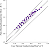 |
Figure 6 Parity plot of experimental vs. predicted thermal conductivity values using the XGBoost-based model combined with equation (10) for four jet fuels at 0.1 MPa and temperatures ranging from 253 K to 373 K. Experimental data were collected from the work by Malatesta and Yang [2]. The dashed line stands for the bisector of the diagram surrounded by two dotted lines corresponding to a 5% uncertainty. |
As a final validation for our approach, predictions were made for jet fuels. For this purpose, it is necessary to simplify fuels to surrogates. According to previous work [5], fuels were characterized using outputs of two-dimensional gas chromatography (GC × GC) which is able to provide detailed information about a fuel chemical composition. Fuel compositions were expressed as mass fraction distributions vs. number of carbon atoms for different hydrocarbon families such as paraffins, naphthenes, and aromatics. A representative molecular structure is then attributed to each family/number of carbon atoms bin [5], resulting in a fuel surrogate containing up to 74 compounds. Four jet fuel (three JP-5 and one F-24) compositions were collected from the work by Malatesta and Yang [2]. Figure 4 presents the parity plot comparing experimental vs. predicted thermal conductivity values for the four jet fuels. An overall MAE of 2.9% was observed, with MAEs ranging from 1.2% to 4.4% for individual jet fuels, which compares well with Malatesta and Yang’s predictions [2]. Data points roughly remain in the 5% uncertainty interval. Our approach combining the XGBoost-based model with equation (10) appears to systematically overestimate experimental data, while this trend was not observed on Figures 4 and 5. One possible explanation lies in the selection of representative components for each family/number of carbon atoms bin, which may not be the most appropriate technique in this context, leaving room for future improvements.
4 Conclusion
In this work, we applied Machine Learning techniques to develop a fully predictive approach to estimate the thermal conductivity of mixtures containing hydrocarbons and oxygenated compounds in the liquid phase at atmospheric pressure. The work was divided into different tasks, starting with a compilation of experimental data, followed by a careful data curation. Datasets were constructed containing information for pure compounds and binary mixtures. The binary mixture dataset was used in a symbolic regression-based strategy to generate mixing rules considering different scenarios and five independent data manipulation strategies. Subsequently, using the pure compound dataset, new quantitative structure property relationship models were developed and benchmarked with work recently published in the literature. The newly developed QSPR models were used to power mixing rules generated with symbolic regression to predict thermal conductivity values of binary mixtures. A mixing rule was then designed to propose a potential extension to multi-component – two or more components – mixtures and first assessed on ternary and quaternary mixtures. The comparisons showed good agreement between predicted values and available experimental data. Then, the approach has shown its full potential in accurately predicting thermal conductivity values for jet fuels for temperatures ranging from 253 K to 373 K.
Performed comparisons across our datasets first demonstrate that symbolic regression is an interesting tool to derive mixing rules, then mixing rules based on power-law models are recommended for the calculation of thermal conductivity of mixture, more precisely for non-aqueous systems. Additionally, they validated that our hybrid model, combining QSPR modeling and mixing rules generated with symbolic regression, can be used for the prediction of thermal conductivity values for pure compounds and mixtures at temperatures that are not yet covered experimentally in the literature. Future work could consider incorporating pressure effects to improve the applicability of the models, although up to 50–60 bar, the effect of pressure on the thermal conductivity of liquids is generally neglected. More generally, the approach implemented in this work can be extended to other properties falling within the framework of jet fuel specifications.
Data availability statement
The authors do not have permission to share experimental data.
Supplementary material
Supplementary material contains the best mixing rule expressions, extracts of predicted thermal conductivity values for DB samples, for ternary mixtures, for quaternary mixtures, and predictions made for jet fuels. Access Supplementary Material
References
- Gan C., Ma Q., Bao S., Wang X., Qiu T., Ding S. (2023) Discussion of the standards system for sustainable aviation fuels: an aero-engine safety perspective, Sustainability 15, 24, 16905. https://doi.org/10.3390/su152416905. [Google Scholar]
- Malatesta W.A., Yang B. (2021) Aviation Turbine Fuel Thermal Conductivity: A Predictive Approach Using Entropy Scaling-Guided Machine Learning with Experimental Validation, ACS Omega 6, 43, 28579–28586. https://doi.org/10.1021/acsomega.1c02934. [Google Scholar]
- Moreno Jimenez R., Creton B., Marre S. (2023) Machine learning-based models for accessing thermal conductivity of liquids at different temperature conditions, SAR and QSAR in Environmental Research 34, 8, 605–617. https://doi.org/10.1080/1062936X.2023.2244410. [Google Scholar]
- Saldana D.A., Starck L., Mougin P., Rousseau B., Pidol L., Jeuland N., Creton B. (2011) Flash point and cetane number predictions for fuel compounds using Quantitative Structure Property Relationship (QSPR) methods, Energy Fuels 25, 9, 3900–3908. https://doi.org/10.1021/ef200795j. [Google Scholar]
- Creton B., Brassart N., Herbaut A., Matrat M. (2024) Numerical approaches to determine cetane number of hydrocarbons and oxygenated compounds, Mixtures, and their Blends, Energy & Fuels 38, 16, 15652–15661. https://doi.org/10.1021/acs.energyfuels.4c03007. [Google Scholar]
- Boehm C., Yang Z., Bell D.C., Faulhaber C., Mayhew E., Bauder U., Eckel G., Heyne J.S. (2024), Perspective on Fuel Property Blending Rules for Design and Qualification of Aviation Fuels: A Review, Energy Fuels 38, 18, 17128–17145. https://doi.org/10.1021/acs.energyfuels.4c02457. [Google Scholar]
- Shao Y., Yu M., Zhao M., Xue K., Zhang X., Zou J.J., Pan L. (2025) Comprehensive accurate prediction of critical jet fuel properties with multiple machine learning models, Chemical Engineering Science 304, 121018. https://doi.org/10.1016/j.ces.2024.121018. [Google Scholar]
- Dehlouz A., Jaubert J.-N., Galliero G., Bonnissel M., Privat R. (2022) Combining the entropy-scaling concept and cubic- or SAFT equations of state for modelling thermal conductivities of pure fluids, Int. J. Heat Mass Transf. 196, 123286. https://doi.org/10.1016/j.ijheatmasstransfer.2022.123286 [Google Scholar]
- Hopp M., Gross J. (2019) Thermal conductivity from entropy scaling: a group-contribution method, Indus. Eng. Chem. Res. 58, 44, 20441–20449. https://doi.org/10.1021/acs.iecr.9b04289. [Google Scholar]
- Khosharay S., Khosharay K., Di Nicola G., Pierantozzi M. (2017) Modelling investigation on the thermal conductivity of pure liquid, vapour, and supercritical refrigerants and their mixtures by using Heyen EOS, Phys. Chem. Liquids 56, 1, 124–140. https://doi.org/10.1080/00319104.2017.1306859. [Google Scholar]
- Gaitonde U.N., Deshpande D.D., Sukhatme S.P. (1978) The thermal conductivity of liquid mixtures, Ind. Eng. Chem. Fundam. 17, 4, 321–325. https://doi.org/10.1021/i160068a018. [Google Scholar]
- Filippov L.P., Novoselova N.S. (1955) The thermal conductivity of solutions of normal liquid, Vest. Mask. Gos. Univ. Ser. Fiz. 10, 3, 37–40. [Google Scholar]
- Filippov L.P. (1968) Liquid thermal conductivity research at Moscow University, Int. J. Heat Mass Transf. 11, 2, 331–345. https://doi.org/10.1016/0017-9310(68)90161-0. [Google Scholar]
- Jamieson D.T., Irving J.B. (1974) Report No. NEL 567, National Engineering Laboratory, Glasgow. [Google Scholar]
- McLaughlin E. (1964) The thermal conductivity of liquids and dense gases, Chem. Rev. 64, 4, 389–428. https://doi.org/10.1021/cr60230a003. [Google Scholar]
- Poling B.E., Prausnitz J.M., O’Connell J.P. (2001) The properties of gases and liquids, 5 ed. New York: McGraw-Hill. https://doi.org/10.1036/0070116822. [Google Scholar]
- Davies A., Veličković P., Buesing L., Blackwell S., Zheng D., Tomašev N., Tanburn R., Battaglia P., Blundell C., Juhász A., Lackenby M., Williamson G., Hassabis D., Kohli P. (2021) Advancing mathematics by guiding human intuition with AI, Nature 600, 70–74. https://doi.org/10.1038/s41586-021-04086-x. [NASA ADS] [CrossRef] [Google Scholar]
- Koza J.R. (1994) Genetic programming as a means for programming computers by natural selection, Stat. Comput. 4, 87–112. https://doi.org/10.1007/BF00175355. [Google Scholar]
- Angelis D., Sofos F., Karakasidis T. E. (2024) Reassessing the transport properties of fluids: A symbolic regression approach, Phys. Rev. E 109, 015105. https://doi.org/10.1103/PhysRevE.109.015105. [Google Scholar]
- Makke N., Chawla S. (2024) Interpretable scientific discovery with symbolic regression: a review, Artif. Intell. Rev. 57, 2. https://doi.org/10.1007/s10462-023-10622-0. [Google Scholar]
- Seifert L., Leuchtenberger-Engel L., Hopmann C. (2024) Enhancing the quality of polypropylene recyclates: predictive modelling of the melt flow rate and shear viscosity, Polymers 16, 2326. https://doi.org/10.3390/polym16162326. [Google Scholar]
- Nieto-Draghi C., Fayet G., Creton B., Rozanska X., Rotureau P., de Hemptinne J.-C., Ungerer P., Rousseau B., Adamo C. (2015) A general guidebook for the theoretical prediction of physicochemical properties of chemicals for regulatory purposes, Chem. Rev. 115, 13093–13164. https://doi:10.1021/acs.chemrev.5b00215. [Google Scholar]
- Cheméo, Chemical properties database available from: https://www.chemeo.com/ (accessed in 2025). [Google Scholar]
- Korea Thermophysical Properties Data Bank (KDB) http://www.cheric.org/research/tech/periodicals/ (accessed in 2025). [Google Scholar]
- National Institute of Standards and Technology (NIST) – NIST Standard Reference Database Number 69. https://doi.org/10.18434/T4D303. [Google Scholar]
- Ilten D.F. (1991) DETHERM: Thermophysical property data for the optimization of heat-transfer equipment, J. Chem. Inform. Comput. Sci. 31, 1, 160–167. https://doi.org/10.1021/ci00001a029. [Google Scholar]
- Bloxham J.C., Redd M.E., Giles N.F., Knotts T.A., Wilding W.V. (2021) Proper use of the DIPPR 801 database for creation of models, methods, and processes, J. Chem. Eng. Data 66, 1, 3–10. https://doi.org/10.1021/acs.jced.0c00641. [Google Scholar]
- Dobbelaere M.R., Plehiers P.P., Van de Vijver R., Stevens C.V., Van Geem K.M. (2021) Learning molecular representations for thermochemistry prediction of cyclic hydrocarbons and oxygenates, J. Phys. Chem. A 125, 23, 5166–5179. https://doi.org/10.1021/acs.jpca.1c01956. [Google Scholar]
- Tosco P., Stiefl N., Landrum G. (2014) Bringing the MMFF force field to the RDKit: implementation and validation, J. Cheminform. 6, 1, 37. https://doi.org/10.1186/s13321-014-0037-3. [Google Scholar]
- RDKit: Cheminformatics and Machine Learning Software. (2013) http://www.rdkit.org. [Google Scholar]
- Cranmer M.D., (2023) Interpretable machine learning for science with PySR and SymbolicRegression.jl, arXiv preprint arXiv:2305.01582. https://doi.org/10.48550/arXiv.2305.01582. [Google Scholar]
- Muratov E.N., Varlamova E.V., Artemenko A.G., Polishchuk P.G., Kuz’Min V.E. (2012) Existing and developing approaches for QSAR analysis of mixtures, Molecular Inform. 31, 3-4, 202–221. https://doi.org/10.1002/minf.201100129. [Google Scholar]
- Venegas-Reynoso A., Creton C., Giarracca-Mehl L., Lacoue-Negre M., Ruckebusch C., Duponchel L. (2025) Oxidation stability of hydrocarbons: a machine-learning-based study, Energy Fuels 39, 9, 4361–4373. https://doi.org/10.1021/acs.energyfuels.4c04926. [Google Scholar]
- Ramos-Pallares F., Schoeggl F.F., Taylor S.D., Yarranton H.W. (2018) Expanded fluid-based thermal conductivity model for hydrocarbons and crude oils, Fuel 224, 68–84. https://doi.org/10.1016/j.fuel.2018.03.060. [Google Scholar]
All Tables
R 2 and RMSE (in W m−1 K−1) values calculated for the different PySR-generated mixing rules when applied to SDB1 Training and Test sets.
Performances of SVR and XGBoost-based QSPR models when applied to SDB2 Test sets. The last column reports R2 values when QSPR models are used to predict compounds involved in mixtures of the SDB1 dataset.
R 2, RMSE (in W m−1 K−1), and MAE (in W m−1 K−1) values calculated for the different mixing rules powered with the three QSPR models, when applied to the DB dataset.
All Figures
|
Figure 1 Distributions of hydrocarbons (black) and oxygenated compounds (dark grey) within the databases. Filled bars stand for samples in the DB database, and dashed bars stand for mixtures in the SDB1 dataset. The values above bars indicate the number of compounds in each chemical subfamily. |
| In the text | |
|
Figure 2 Projections of mixture samples into the space formed by t-SNE1, t-SNE2, and t-SNE3. Blue and red symbols stand for mixtures in the DB database and in the SDB1 dataset, respectively. t-SNE1, t-SNE2 and t-SNE3 are unitless. |
| In the text | |
|
Figure 3 Illustration of the tree-like architecture representation. X stands for descriptors or variables. |
| In the text | |
|
Figure 4 Parity plot of experimental vs. predicted thermal conductivity values using the XGBoost-based model combined with equation (10) for ternary mixtures, with temperatures ranging from 280 K to 360 K. The dashed line stands for the bisector of the diagram surrounded by two dotted lines corresponding to a 5% uncertainty. |
| In the text | |
|
Figure 5 Parity plot of experimental vs. predicted thermal conductivity values using the XGBoost-based model combined with equation (10) for quaternary mixtures, with temperatures ranging from 280 K to 360 K. The dashed line stands for the bisector of the diagram surrounded by two dotted lines corresponding to a 5% uncertainty. |
| In the text | |
|
Figure 6 Parity plot of experimental vs. predicted thermal conductivity values using the XGBoost-based model combined with equation (10) for four jet fuels at 0.1 MPa and temperatures ranging from 253 K to 373 K. Experimental data were collected from the work by Malatesta and Yang [2]. The dashed line stands for the bisector of the diagram surrounded by two dotted lines corresponding to a 5% uncertainty. |
| In the text | |
Current usage metrics show cumulative count of Article Views (full-text article views including HTML views, PDF and ePub downloads, according to the available data) and Abstracts Views on Vision4Press platform.
Data correspond to usage on the plateform after 2015. The current usage metrics is available 48-96 hours after online publication and is updated daily on week days.
Initial download of the metrics may take a while.