")
")
| Issue |
Sci. Tech. Energ. Transition
Volume 78, 2023
Power Components For Electric Vehicles
|
|
|---|---|---|
| Article Number | 41 | |
| Number of page(s) | 10 | |
| DOI | https://doi.org/10.2516/stet/2023037 | |
| Published online | 22 décembre 2023 | |
Regular Article
Multi-material topology optimization of a flux switching machine
1
Université Paris-Saclay, ENS Paris-Saclay, CNRS, SATIE, 4, Avenue des Sciences, 91190 Gif-sur-Yvette, France
2
CY Cergy Paris Université, CNRS, SATIE, site de de Neuville, 5 mail Gay Lussac, 95031 Neuville sur Oise, France
3
CNAM, LMSSC, Case 2D6R10, 2 rue Conté, 75003 Paris, France
4
Université Paris Saclay, ENS Paris Saclay, CentraleSupélec, CNRS, LMPS, 91190 Gif-sur-Yvette, France
5
ENS Rennes, CNRS, SATIE, Campus de Ker Lann, 11 Av. Robert Schuman, 35170 Bruz, France
* Corresponding author: Cette adresse e-mail est protégée contre les robots spammeurs. Vous devez activer le JavaScript pour la visualiser.
Received:
14
September
2023
Accepted:
8
November
2023
Abstract
This paper investigates the topology optimization of the rotor of a 3-phase flux-switching machine with 12 permanent magnets located within the stator. The objective is to find the steel distribution within the rotor that maximizes the average torque for a given stator, permanent magnets, and electrical currents. The optimization algorithm relies on a density method based on gradient descent. The adjoint variable method is used to compute the sensitivities efficiently. Since the rotor topology depends on the current feedings, this approach is tested on several electrical periods and returns alternative topologies. Then, the method is extended to the multi-material case and applied to optimize the non-magnet part of the stator. When dealing with 3 phases, the algorithm returns the reference topology as well as a theoretical machine with no return conductor according to the set current angle. To illustrate the creativity of the method, the optimization is finally performed with a single-phase and returns a new topology.
Key words: Density method / Flux switching machine / Multi-material topology optimization / Nonlinear magnetostatics
© The Author(s), published by EDP Sciences, 2023
 This is an Open Access article distributed under the terms of the Creative Commons Attribution License (https://creativecommons.org/licenses/by/4.0), which permits unrestricted use, distribution, and reproduction in any medium, provided the original work is properly cited.
1 Introduction
Topology optimization is a conception tool that makes no use of geometric parametrization. It was first developed in mechanical engineering by [1], then introduced in electrical engineering by [2], and has gained interest from engineers in the last decade with the development of additive manufacturing [3]. Among various techniques, such as the level-set method [4], or the phase-field approach [5] (see [6] for a recent overview), density-based approaches [1, 7] are the most popular. The principle of this technique is explained hereafter.
The geometry to be optimized is represented by a so-called density field ρ, which can be interpreted as pixelation on Ne elements once discretized spatially, as shown in Figure 1. A density value of 0 represents air, and 1 represents iron in the corresponding mesh. The topology optimization problem then reads as![Mathematical equation: $$ \begin{array}{cc}\mathrm{find}& {{\rho }}_{\mathrm{opt}}=\mathrm{arg}\mathrm{min}f\left({\rho }\right)\\ \mathrm{subject}\enspace \mathrm{to}& {\rho }\in [\mathrm{0,1}{]}^{{N}_e},\end{array} $$](/articles/stet/full_html/2023/01/stet20230172/stet20230172-eq1.gif) (1)where f is the objective function to minimize (such as the cost, the mass, or in the present case the opposite of the average torque), and ρ is the vector of optimization variables, which contains the density of each mesh element. To avoid solving a combinatorial problem that may be intractable, density methods introduce intermediate materials (also called gray materials) associated with density values strictly between 0 and 1. Therefore, the material properties can be continuously interpolated between the actual candidate materials to use a fast gradient-based optimization algorithm.
(1)where f is the objective function to minimize (such as the cost, the mass, or in the present case the opposite of the average torque), and ρ is the vector of optimization variables, which contains the density of each mesh element. To avoid solving a combinatorial problem that may be intractable, density methods introduce intermediate materials (also called gray materials) associated with density values strictly between 0 and 1. Therefore, the material properties can be continuously interpolated between the actual candidate materials to use a fast gradient-based optimization algorithm.
 |
Fig. 1 Principle of density-based representation. a) Original domain, b) Density-based representation. |
Although the presence of gray materials is not critical during optimization, they should not appear in the final geometry. Indeed, gray materials do not necessarily have a proper physical interpretation or may represent, in the best case, a microstructure that is complex to manufacture [8]. A common solution for removing gray materials proposed by the literature involves penalizing the material interpolation, such as the Solid Isotropic Materials with Penalization (SIMP) scheme [8, 9]. Yet topology optimization problems are generally ill-posed, and other numerical artifacts can occur, such as checkerboards that need regularization (e.g., numerical filtering [10]). Density-based approaches have been applied to many magnetics problems, from the simple C-core electromagnets [11, 12] to 3-phase synchronous reluctant machines with several materials and physics [13, 14]. However, apart from [15], no such work has studied unconventional structures such as Flux Switching Machines (FSM), where the unbiased creativity of topology optimization may be the most useful.
This article aims to apply a density-based topology optimization methodology to FSM. First proposed by [16], this type of machine contains a passive rotor with the field inductor located in the stator only, making its cooling easier [17] and suitable for high-speed applications. Several types of FSM exist in the literature; see [18]. The chosen test case is a 3-phase Permanent Magnet Flux Switching (PMFS) machine with 12 permanent magnets evenly spaced within the stator, adapted from [19] and shown in Figure 2.
This paper is structured as follows. First, Section 2 recalls the magnetostatics equations. The optimization algorithm is then detailed in Section 3. Next, two numerical applications exploring unconventional topologies are presented and discussed. On the one hand, classical rotor optimizations are conducted under various electrical frequencies in Section 4. On the other hand, stator optimization, which requires a multi-material framework, explores the topologies obtained with 1 and 3-phase current feeding in Section 5. In conclusion, Section 6 summarizes the essential results and draws perspectives on this work.
2 Physical problem
Since density-based topology optimization will be used, we first set up the interpolations of material properties in Section 2.1 in the Kennelly convention [20]. These quantities were then injected in the physical equation of magnetostatics recalled in Section 2.2, which is further discretized with the 2D Finite Element Method (FEM).
2.1 Material interpolation
There are at least two material properties of interest when dealing with a magnetostatics problem: the magnetic polarization of materials m1 and the current density. In the case of soft magnetic material, m is collinear to the flux density b and 0 when b = 0, so that it can be expressed in terms of a scalar reluctivity ν(b) (2)
(2)
Two possibilities are generally reported in the literature to interpolate the magnetic properties when dealing with soft magnetic materials. One can interpolate either the magnetic reluctivity ν as in [12, 21, 22], or the magnetic permeability μ = ν−1 as in [2, 23, 24], among many others. However, an additional magnetic quantity to interpolate (the remanence) should be introduced when dealing with polarized materials, as in [24, 25]. We choose an alternative, proposed in [26], which interpolates the magnetic polarization  of a FeCo alloy (AFK1 from Aperam [27]) directly. The corresponding BH curve is plotted in Figure 3. Its interpolation reads in the general case of nm materials
 (3)where Pm is a penalization function associated with the magnetic polarization, ωi a shape function defined in [28] associated with the i-vertex of a convex interpolation domain
  , and mi the magnetic polarization of the i-material. To address the topology optimization of the stator, the current density should also be interpolated with a similar scheme:
 (4)where Pj is a penalization function associated with the current density, and ji, is the out-of-plane component of the current density of the material i. The chosen domain
  as well as the penalization functions are given in Sections 4 and 5, and an example of interpolation is drawn in Figure 4. More details on the interpolation scheme and associated algorithms can be found in [29].
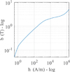 |
Fig. 3 Anhysteretic BH curve of FeCo in logarithmic scale used for the computations. |
 |
Fig. 4 Interpolation example of the current density amplitude between 7 materials. Note that in the real optimization problem in Section 5, the actual value of the current density at each electric angle is interpolated instead of its amplitude. |
2.2 Physical equations
From the static Maxwell’s equations, one can write the magnetostatics equation for a 2D problem [26]: (5)with
  and
and  the x and y components of the interpolated magnetic polarization
  ,
,  the current density, and az the z-component of the magnetic vector potential a, related to the flux density by the formula b = ∇ × a. To be solved numerically, the strong equation (5) should be written in a weak form and discretized using, for instance, the FEM. Then, the physical problem reads as follows
 (6)where K is the finite element matrix, a the vector containing the discretized degrees of freedom az, and s right-hand side related to source terms. Figure 5 draws the mesh used in this article. Homogeneous Dirichlet boundary conditions confined the flux inside the machine, and a locked-step sliding band technique [30] is applied to emulate the rotation of the rotor without remeshing.
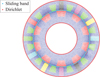 |
Fig. 5 Mesh of the simulation domain containing 30,666 first-order elements and 16,329 nodes. |
The nonlinear FEM system (6) is solved with the Newton-Raphson scheme: (7)with rn = Kan − s(ρ, an) is the residual of (6) at iteration n. After convergence, the torque can be computed from the flux density field within the airgap e by Arkkio’s method [31]:
 (8)where br, bθ are the cylindrical components of the flux density, and Rs and Rr are the stator’s inner radius and the rotor’s outer radius, respectively. The axial length of the machine is normalized to L = 1 m.
3 Optimization algorithm
The purpose of the optimization is to solve the problem (1), i.e. to find an optimal density vector ρ that minimizes a given objective function f. In this article, the objective function is set to the opposite of the average torque (i.e., the average torque should be maximized), computed with (8) over 720 angular positions along one mechanical turn: (9)
(9)
As the density vector ρ contains many components (at least one per mesh element), the optimization algorithm should rely on the sensitivity dρf. The optimization flowchart is given in Figure 6.
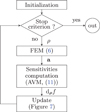 |
Fig. 6 Flowchart of the optimization algorithm. |
The efficient computation of dρf components is non-trivial since f rarely depends on ρ explicitly. Actually, f rather depends on the system’s physical state, such as the magnetic field b in the present case. The latter depends implicitly on the density vector ρ through the physical equation (6), which involves the material interpolations (3) and (4).
3.1 Sensitivities computation
The Adjoint Variable Method (AVM) is the most efficient approach to compute first-order derivatives from many variables. Once the FEM system (6) is solved, the sensitivities are computed using the adjoint state λ, which is the solution of the following adjoint system (10)then the sensitivities with respect to each design variable ρi can be calculated with
 (11)
(11)
Note that (10) is linear and should be solved only once per iteration. Consequently, the average single-thread computing time per optimization iteration of the sensitivities (41s) is almost negligible compared to the one of the nonlinear FEM (352s). This high computing time is caused by the high number of nodes and angular positions for the calculation.
3.2 Update
To accelerate the optimization to the real materials, each component  of the descent direction associated with the mesh element
  is normalized as follows:
 (12)with
  the sensitivity vector of f to the part of the global density vector associated with the element
  . A simplified trust-region algorithm [32] adapts the step size heuristically according to a quality indicator, which compares the measured variation of the objective function Δf between two consecutive iterations with its variation predicted by the linearized model. It is defined as
 (13)where Δρ is the variation of the density vector between two consecutive iterations. If q is too low, the iteration is rejected, and the step size is reduced. If q is big enough, the iteration is accepted, and the step size can also be increased. The flowchart in Figure 7 gives more details on this algorithm that is applied in the following sections.
 |
Fig. 7 Flowchart of the update algorithm. |
Then, ρn+1 is projected orthogonally to remain within the bounds of  . The algorithm stops if the step α becomes smaller than 5 × 10⁻⁴, or after 100 iterations.
4 Rotor optimization
The presented topology optimization algorithm is first applied to FSM rotor. The optimization domain is shown in Figure 8. In order to explore new structures, different electrical frequencies are injected within the FSM. The optimization setup is presented in Section 4.1, and the results in Section 4.2.
 |
Fig. 8 Optimization domain (gray) in case of a rotor optimization. |
4.1 Parametrization
There are only two candidate materials to distribute inside the rotor: soft magnetic steel (FeCo alloy AFK1 from Aperam [27]) and air. Therefore, the interpolation domain  is a 1D line segment that joins both materials and supports the optimization variables contained in ρ; air corresponding to ρ = 0 and steel to ρ = 1. The density interpolates the magnetic polarization linearly:
![Mathematical equation: $$ \mathop{m}\limits^\tilde:\left\{\begin{array}{c}\left(\mathcal{D}=\left[\mathrm{0,1}\right]\right)\times {\mathbb{R}}^2\to {\mathbb{R}}^2\\ \rho,{b}\mapsto \rho \enspace {{m}}_{{FeCo}}\left({b}\right),\end{array}\right. $$](/articles/stet/full_html/2023/01/stet20230172/stet20230172-eq27.gif) (14)and the resulting BH curves for intermediate materials are given in Figure 9. Note that the intermediate BH curves are equivalent to those of a 1D serial assembly of steel and air along the flux lines, ρ representing the linear fraction of steel2. Initially, all densities are set to 0.5.
(14)and the resulting BH curves for intermediate materials are given in Figure 9. Note that the intermediate BH curves are equivalent to those of a 1D serial assembly of steel and air along the flux lines, ρ representing the linear fraction of steel2. Initially, all densities are set to 0.5.
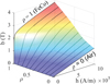 |
Fig. 9 Magnetic behavior used for the computation. |
Because there is no current neither in air nor steel, the current density inside the rotor  is set to 0. However, the current density inside a stator conductor
  , following the enumeration in Table 1, reads:
![Mathematical equation: $$ {j}_i=J\mathrm{cos}\left(N{\theta }_m-i\frac{\pi }{3}+\psi \right),\hspace{1em}\enspace i\in [[ \mathrm{0,5}]], $$](/articles/stet/full_html/2023/01/stet20230172/stet20230172-eq30.gif) (15)where J = 10 A/mm2 is the current density amplitude, N is the number of electrical periods during one complete mechanical rotation, θm is the mechanical angle of the rotor, and ψ the electric angle set to 0° for the rotor optimization. The N values were tested between 1 and 20, corresponding to different electrical frequencies.
(15)where J = 10 A/mm2 is the current density amplitude, N is the number of electrical periods during one complete mechanical rotation, θm is the mechanical angle of the rotor, and ψ the electric angle set to 0° for the rotor optimization. The N values were tested between 1 and 20, corresponding to different electrical frequencies.
Materials names and indices.
4.2 Results
The final average torques of optimized machines are plotted in Figure 10. The highest torque is obtained for N = 10, corresponding to the current feeding of the reference machine shown in Figure 2. Therefore, a very similar rotor design shown in Figure 11a is obtained and develops about the same torque (〈T10〉 = 2244 Nm/m) as the reference one (〈Tref〉 = 2236 Nm/m) under the same current feeding.
 |
Fig. 10 Average torque of optimized designs depending on N. |
 |
Fig. 11 Resulting designs and flux maps with the highest torques for rotor optimization [15]. a) Final design N = 0, b) Flux density (N = 10), c) Final design N = 4, d) Flux density (N = 4), e) Final design N = 16, b) Flux density (N = 16). |
The results indicated in Figure 10 show that N = 4 and N = 16 can produce a lower torque than the reference but more significant than the rest of the N values. The associated designs are drawn in Figures 11c and 11e, and their convergence curves are compared to the one obtained with an unsuitable value N = 13 in Figures 12a and 12b. Although they reach a lower torque than the N = 10 structure, their topologies fundamentally differ from the reference rotor and are unusual for a human designer. Indeed, they contain disconnected parts, illustrating the ability of topology optimization to find innovative designs.
 |
Fig. 12 Convergence curves during the optimization. a) Torque evolution, b) Step size evolution. |
The algorithm fails to find meaningful structures for the rest of the N values, which may indicate the impossibility of designing suitable rotors under these conditions. An example of such a “bad” optimized design for N = 13 is drawn in Figure 13, which leads to the conjecture that there exist suitable rotors only for N = 4 + 6n, n ∈ N.
 |
Fig. 13 “Bad” structure obtained with N = 13. a) Final design, b) Flux density. |
5 Stator optimization
Density-based methods can be extended to multi-material problems, such as optimizing an FSM stator. Following the results of the previous section, we impose N = 10 with the reference rotor geometry shown in Figure 2. The magnets’ positions and orientations are also fixed, given the optimization zone drawn in Figure 14.
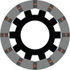 |
Fig. 14 Design domain (gray) in case of the stator optimization. |
5.1 Three-phase machine
The optimization of a 3-phase stator is first addressed. Since the permanent magnets are imposed, there are 8 candidate materials (steel, air, and conductors3) listed in Table 1. A multi-material interpolation formalism is necessary to address this problem. To handle this large amount of materials, the interpolations (3) and (4) are supported by a multidimensional space  . We chose
  as a convex polytope that supports shape functions set {ωi}i∈⟦0,7⟧ [28], represented in Figure 15. The diamond-shaped domain allows the distribution of the conductors onto the same plane with respect to their electrical phase. The basis function values are computed with an optimized version of the code given in [33], available at [34].
 |
Fig. 15 Interpolation domain |

The chosen penalization functions Pm and Pj are adapted from [35] and read:![Mathematical equation: $$ {P}_m:\left\{\begin{array}{c}\left[\mathrm{0,1}\right]\to \left[\mathrm{0,1}\right]\\ \omega \mapsto 1-\frac{1-\omega }{4-3\left(1-\omega \right)},\end{array}\right. $$](/articles/stet/full_html/2023/01/stet20230172/stet20230172-eq33.gif) (16)
(16)
![Mathematical equation: $$ {P}_j:\left\{\begin{array}{c}\left[\mathrm{0,1}\right]\to \left[\mathrm{0,1}\right]\\ \omega \mapsto \frac{\omega }{2-\omega }.\end{array}\right. $$](/articles/stet/full_html/2023/01/stet20230172/stet20230172-eq34.gif) (17)
(17)
The optimization is then performed for several current angles ψ ∈ [0°, 60°]. The resulting designs are given in Figure 16 with their average torques. The current angle strongly influences the resulting topologies; when it is incorrectly set, it may return non-manufacturable designs with no return conductors.
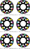 |
Fig. 16 Designs obtained after stator optimizations. a) ψ = 0°, 〈T〉 = 2444 Nm/m, b) ψ = 12°, 〈T〉 = 2522 Nm/m, c) ψ = 24°, 〈T〉 = 2747 Nm/m, d) ψ = 36°, 〈T〉 = 2798 Nm/m, e) ψ = 48°, 〈T〉 = 2643 Nm/m, f) ψ = 60°, 〈T〉 = 2444 Nm/m. |
Intermediate ψ values promote single conductors in each slot, as there is a factor  between the total current amplitude in sliced conductors and plain conductor slots, as illustrated in Figure 17.
 |
Fig. 17 Fresnel diagram of the current in sliced (black) and plain conductors (red). |
The structure obtained with ψ = 0° is very similar to the reference shown in Figure 2. However, the conductors are larger, carrying more current for the same current density, set to J = 10 A/mm2. Consequently, the average torque of the optimized design is higher. Note that the order of conductors is inverted within the same slot. As topology optimization considers only electromagnetism performance, it places the conductors according to their electrical phase, resulting in distributed windings. However, Figure 2 proposes concentrated windings, probably for manufacturability reasons that are still ongoing research topics in topology optimization.
5.2 Single-phase machine
To illustrate the creativity of topology optimization, we now address an academic problem with no reference solution. More precisely, we want to optimize the stator of a 10/12 machine that has the same 10-tooth rotor and 12-magnet configuration, using only a single electrical phase, i.e., a positive and a negative conductor denoted as  and
and  . Single-phase FSMs are of interest for domestic and low-cost applications, and some classic topologies were compared in [36].
Since there are now only 4 candidate materials, the interpolation domain  is a tetrahedron drawn in Figure 18a, and the basis functions are the barycentric coordinates as illustrated in Figure 18b. The penalization functions are the same as in Section 5.1.
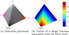 |
Fig. 18 Interpolation domain |

A parametric sweep on ψ was performed. The results are shown in Figure 19, and the corresponding torques are plotted in Figure 20. The case of ψ = 0° [60°] leads to manufacturable designs that reach 2200 Nm/m with a mixture of C- and E-core patterns [37, 38].
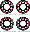 |
Fig. 19 Examples of single-phase optimized designs. a) ψ = 0°, 〈T〉 = 2200 Nm/m, b) ψ = 20°, 〈T〉 = 2200 Nm/m, c) ψ = 40°, 〈T〉 = 2198 Nm/m, d) ψ = 60°, 〈T〉 = 2198 Nm/m. |
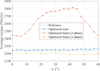 |
Fig. 20 Average torque obtained for each ψ. |
5.3 Torque comparison
The dependence of the average torque with the current angle ψ is given in Figure 20 hereafter.
The rotor is almost insensitive to ψ because its optimized topology compensates for the electric phase shift by a mechanical rotation. This mechanical rotation is impossible for the stator optimization since the permanent magnet positions are imposed. For the three-phase machine, the factor between the maximum and minimum average torque is  because of the sliced conductors, as predicted in Section 5.1. Since there are no sliced conductors within the stator slots for the single-phase machine structures, its average torque remains almost constant.
Even if it was not considered in the optimization, the torque ripple  is an important criterion when designing an electrical machine, and is given in Table 2. The corresponding instant torques of manufacturable machines (i.e., the structures obtained with ψ = 0°) are plotted in Figure 21.
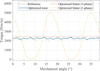 |
Fig. 21 Instant torque obtained for the optimized designs for each ψ. |
Torques of the optimized designs (ψ = 0°).
The single-phase machine produces a pulsating torque with a high ripple but can still produce a significant average torque. The two other optimized designs outperform the reference, and the best performance is obtained by optimizing the 3-phase stator.
In the end, the best-found topology is similar to the reference, but our topology optimization approach has explored other unusual structures.
6 Conclusion
This work presents and details a density-based topology optimization method applied to the torque maximization of a permanent magnet flux switching machine. Unconventional problems are addressed, such as the rotor optimization for several electrical frequencies and the stator optimization for different numbers of phases. Unusual structures were obtained, such as disconnected rotors or a hybrid single-phase stator made of C- and E-cores. This variety of results from an empty optimization domain highlights the creativity and unbiasedness of a topology optimization approach. The best-obtained topology is similar to the reference design but with better torque performances. In other applications, the optimal topology might differ from the known references.
In conclusion, topology optimization is a valuable tool to help design electrical machines that can be improved further. Future research will add the permanent magnet to the set of candidate materials so that the stator can be optimized in its entirety. Such work will be the first step to the topology optimization of a complete flux switching machine with both rotor and stator simultaneously. Additional objective functions can be added to tackle industrial problems such as ripple and back-electromotive force. Finally, other physics such as thermics and mechanics may be considered in order to obtain more ready-to-use designs.
The magnetic polarization (unit T, vector-valued) is often denoted as J in the literature. We adopt the notation m to avoid confusion with the amplitude of the current density.
However, the gray materials are assumed to be isotropic, whereas a serial assembly is not.
The 6 electrical phases (3 positives and 3 negatives) are considered different materials even if they are all made of copper because they do not carry the same current density.
References
- Bendsøe M.P. (1989) Optimal shape design as a material distribution problem, Struct. Optim. 1, 4, 193–202. https://doi.org/10.1007/BF01650949. [CrossRef] [Google Scholar]
- Dyck D.N., Lowther D.A. (1996) Automated design of magnetic devices by optimizing material distribution, IEEE Trans. Magn. 32, 3, 1188–1192. https://doi.org/10.1109/20.497456. [CrossRef] [Google Scholar]
- Zhu J., Zhou H., Wang C., Zhout L., Yuan S., Zhang W. (2021) A review of topology optimization for additive manufacturing: status and challenges, Chinese J. Aeronaut. 34, 1, 91–110. https://doi.org/10.1016/j.cja.2020.09.020. [CrossRef] [MathSciNet] [Google Scholar]
- Kim Y.S., Park I.H. (2010) Topology optimization of rotor in synchronous reluctance motor using level set method and shape design sensitivity, IEEE Trans. Appl. Supercond. 20, 3, 129–133. https://doi.org/10.1109/icems.2013.6754538. [Google Scholar]
- Choi J.S., Izui K., Nishiwaki S., Kawamoto A., Nomura T. (2011) Topology optimization of the stator for minimizing cogging torque of IPM motors, IEEE Trans. Magn. 47, 10, 3024–3027. https://doi.org/10.1109/TMAG.2011.2158572. [CrossRef] [Google Scholar]
- Lucchini F., Torchio R., Cirimele V., Alotto P., Bettini P. (2022) Topology optimization for electromagnetics: a survey, IEEE Access 10, 98593–98611. https://doi.org/10.1109/access.2022.3206368. [CrossRef] [Google Scholar]
- Rozvany G.I.N., Zhou M., Birker T. (1992) Generalized shape optimization without homogenization, Struct. Optim. 4, 3–4, 250–252. https://doi.org/10.1109/AIEEPAS.1955.4499226. [CrossRef] [Google Scholar]
- Bendsøe M.P., Sigmund O. (1999) Material interpolation schemes in topology optimization, Arch. Appl. Mech. 69, 9–10, 635–654. https://doi.org/10.1007/s004190050248. [CrossRef] [Google Scholar]
- Sanogo S., Messine F. (2018) Topology optimization in electromagnetism using SIMP method: issues of material interpolation schemes, COMPEL – Int. J. Comput. Math. Electr. Electron. Eng. 37, 6, 2138–2157. https://doi.org/10.1108/COMPEL-04-2017-0170. [CrossRef] [Google Scholar]
- Sigmund O. (2007) Morphology-based black and white filters for topology optimization, Struct. Multidiscipl. Optim. 33 4–5, 401–424. https://doi.org/10.1007/s00158-006-0087-x. [CrossRef] [Google Scholar]
- Wang S., Kang J. (2002) Topology optimization of nonlinear magnetostatics, IEEE Trans. Magn. 38, 2, 1029–1032. https://doi.org/10.1109/20.996264. [CrossRef] [Google Scholar]
- Choi J.S., Yoo J. (2008) Structural optimization of ferromagnetic materials based on the magnetic reluctivity for magnetic field problems, Comput. Methods Appl. Mech. Eng. 197, 49–50, 4193–4206. https://doi.org/10.1016/j.cma.2008.04.019. [CrossRef] [Google Scholar]
- Guo F., Brown I.P. (2020) Simultaneous magnetic and structural topology optimization of synchronous reluctance machine rotors, IEEE Trans. Magn. 56, 10, 1–12. https://doi.org/10.1109/tmag.2020.3014289. [Google Scholar]
- Lee C., Jang I.G. (2022) Multi-material topology optimization for the PMSMs under the consideration of the MTPA control, Struct. Multidiscipl. Optim. 65, 9, 263. https://doi.org/10.1007/s00158-022-03367-x. [CrossRef] [Google Scholar]
- Cherrière T., Hlioui S., Gabsi M., Laurent L., Louf F., Ahmed H.B. (2022) Topology optimization of flux switching machine rotors, in: Proceedings of the 4th IEEE International Conference on Electrical Sciences and Technologies in Maghreb, CISTEM 2022, 26–28 October, Tunis, Tunisia. https://doi.org/10.1109/CISTEM55808.2022.10044071. [Google Scholar]
- Rauch S.E., Johnson L.J. (1955) Design principles of fluxswitch alternators [includes discussion], Trans. Am. Inst. Electr. Eng. Part 3 74, 3, 1261–1268. https://doi.org/10.1109/AIEEPAS.1955.4499226. [Google Scholar]
- Thomas A.S., Zhu Z.Q., Li G.J. (2014) Thermal modelling of switched flux permanent magnet machines, in: 2014 International Conference on Electrical Machines (ICEM), 2–5 September, Berlin, Germany, pp. 2212–2217. https://doi.org/10.1109/ICELMACH.2014.6960491. [Google Scholar]
- Shi J.T., Zhu Z.Q., Wu D., Liu X. (2016) Comparative study of synchronous machines having permanent magnets in stator, Electr. Power Syst. Res. 133, 304–312. https://doi.org/10.1016/j.epsr.2015.12.018. [CrossRef] [Google Scholar]
- Hoang E., Ahmed H.B., Lucidarme J. (1997) Switching flux permanent magnet polyphased synchronous machines, in: EPE 97, September, Trondheim, pp. 3903–3908. [Google Scholar]
- Coleman J.E. (1973) Conventions for magnetic quantities in SI, Am. J. Phys. 41, 2, 221–223. https://doi.org/10.1119/1.1987179. [CrossRef] [Google Scholar]
- Lee J., Seo J.H., Kikuchi N. (2010) Topology optimization of switched reluctance motors for the desired torque profile, Struct. Multidiscipl. Optim. 42, 5, 783–796. https://doi.org/10.1007/s00158-010-0547-1. [CrossRef] [Google Scholar]
- Seebacher P., Kaltenbacher M., Wein F., Lehmann H. (2020) A pseudo density topology optimization approach in nonlinear electromagnetism applied to a 3D actuator, Int. J. Appl. Electromagn. Mech. 65, 3, 545–559. https://doi.org/10.3233/jae-201501. [Google Scholar]
- Labbé T., Dehez B. (2011) Topology optimization method based on the Maxwell stress tensor for the design of ferromagnetic parts in electromagnetic actuators, IEEE Trans. Magn. 47, 9, 2188–2193. https://doi.org/10.1109/TMAG.2011.2138151. [CrossRef] [Google Scholar]
- Jung T., Lee J., Lee J. (2021) Design and fabrication of magnetic system using multi-material topology optimization, IEEE Access 9, 8649–8658. https://doi.org/10.1109/ACCESS.2021.3049271. [CrossRef] [Google Scholar]
- Gauthey T., Gangl P., Hassan M.H. (2022) Multi-material topology optimization with continuous magnetization direction for motors design, in 25th International Conference on Electrical Machines (ICEM), 5–8 September, Valencia, Spain, IEEE. [Google Scholar]
- Cherrière T., Vancorsellis T., Hlioui S., Laurent L., Louf F., Ahmed H.B., Gabsi M. (2023) A multimaterial topology optimization considering the pm nonlinearity, IEEE Trans. Magn. 59, 5, 1–9. https://doi.org/10.1109/TMAG.2023.3256003. [CrossRef] [Google Scholar]
- Aperam. Iron Cobalt Alloys – IMPHY AFK The electrical revolution. Available at https://www.aperam.com/sites/default/files/documents/imphytek.pdf, last consulted on 13/09/2023. [Google Scholar]
- Wachspress E.L. (1975) A finite element rational basis, volume 114 of Mathematics in Science and Engineering, Academic Press Inc. [Google Scholar]
- Cherrière T., Laurent L., Hlioui S., Louf F., Duysinx P., Geuzaine C., Ahmed H.B., Gabsi M., Fernández E. (2022) Multimaterial topology optimization using Wachspress interpolations for designing a 3-phase electrical machine stator, Struct. Multidiscipl. Optim. 65, 12, 352. https://doi.org/10.1007/s00158-022-03460-1. [CrossRef] [Google Scholar]
- Shi X., Le Menach Y., Ducreux J.-P., Piriou F. (2006) Comparison of slip surface and moving band techniques for modelling movement in 3D with FEM, COMPEL – Int. J. Comput. Math. Electr. Electron. Eng. 25, 1, 17–30. https://doi.org/10.1108/03321640610634290. [CrossRef] [Google Scholar]
- Arkkio A. (1987) Analysis of induction motors based on the numerical solution of the magnetic field and circuit equations, PhD Thesis, Helsinki University of Technology. [Google Scholar]
- Nocedal J., Wright S.J. (2006) Numerical optimization, Springer. [Google Scholar]
- Floater M., Gillette A., Sukumar N. (2014) Gradient bounds for Wachspress coordinates on polytopes, SIAM J. Numer. Anal. 52, 1, 515–532. https://doi.org/10.1137/130925712. [CrossRef] [MathSciNet] [Google Scholar]
- Cherrière T., Laurent L. (2022) Wachspress2d3d, v1.0.0, Zenodo. https://doi.org/10.5281/zenodo.6630215. [Google Scholar]
- Stolpe M., Svanberg K. (2001) An alternative interpolation scheme for minimum compliance topology optimization, Struct. Multidiscipl. Optim. 22, 2, 116–124. https://doi.org/10.1007/s001580100129. [CrossRef] [Google Scholar]
- Jusoh L.I., Sulaiman E., Othman S.M.N.S. (2015) Comparative study of single phase FE, PM and HE flux switching motors, in: 2015 IEEE Student Conference on Research and Development (SCOReD), 13–14 December, Kuala Lumpur, Malaysia. IEEE. [Google Scholar]
- Shen J.-X., Fei W.-Z. (2013) Permanent magnet flux switching machines – topologies, analysis and optimization, in: 4th International Conference on Power Engineering, Energy and Electrical Drives, 13–17 May, Istanbul, Turkey, IEEE. [Google Scholar]
- Min W., Chen J.T., Zhu Z.Q., Zhu Y., Zhang M., Duan G.H. (2011) Optimization and comparison of novel E-core and C-core linear switched flux PM machines, IEEE Trans. Magn. 47, 8, 2134–2141. https://doi.org/10.1109/tmag.2011.2125977. [CrossRef] [Google Scholar]
All Tables
All Figures
|
Fig. 1 Principle of density-based representation. a) Original domain, b) Density-based representation. |
| In the text | |
 |
Fig. 2 Reference PMSF machine adapted from [19]. |
| In the text | |
|
Fig. 3 Anhysteretic BH curve of FeCo in logarithmic scale used for the computations. |
| In the text | |
|
Fig. 4 Interpolation example of the current density amplitude between 7 materials. Note that in the real optimization problem in Section 5, the actual value of the current density at each electric angle is interpolated instead of its amplitude. |
| In the text | |
|
Fig. 5 Mesh of the simulation domain containing 30,666 first-order elements and 16,329 nodes. |
| In the text | |
|
Fig. 6 Flowchart of the optimization algorithm. |
| In the text | |
|
Fig. 7 Flowchart of the update algorithm. |
| In the text | |
|
Fig. 8 Optimization domain (gray) in case of a rotor optimization. |
| In the text | |
|
Fig. 9 Magnetic behavior used for the computation. |
| In the text | |
|
Fig. 10 Average torque of optimized designs depending on N. |
| In the text | |
|
Fig. 11 Resulting designs and flux maps with the highest torques for rotor optimization [15]. a) Final design N = 0, b) Flux density (N = 10), c) Final design N = 4, d) Flux density (N = 4), e) Final design N = 16, b) Flux density (N = 16). |
| In the text | |
|
Fig. 12 Convergence curves during the optimization. a) Torque evolution, b) Step size evolution. |
| In the text | |
|
Fig. 13 “Bad” structure obtained with N = 13. a) Final design, b) Flux density. |
| In the text | |
|
Fig. 14 Design domain (gray) in case of the stator optimization. |
| In the text | |
|
Fig. 15 Interpolation domain |
| In the text | |
|
Fig. 16 Designs obtained after stator optimizations. a) ψ = 0°, 〈T〉 = 2444 Nm/m, b) ψ = 12°, 〈T〉 = 2522 Nm/m, c) ψ = 24°, 〈T〉 = 2747 Nm/m, d) ψ = 36°, 〈T〉 = 2798 Nm/m, e) ψ = 48°, 〈T〉 = 2643 Nm/m, f) ψ = 60°, 〈T〉 = 2444 Nm/m. |
| In the text | |
|
Fig. 17 Fresnel diagram of the current in sliced (black) and plain conductors (red). |
| In the text | |
|
Fig. 18 Interpolation domain |
| In the text | |
|
Fig. 19 Examples of single-phase optimized designs. a) ψ = 0°, 〈T〉 = 2200 Nm/m, b) ψ = 20°, 〈T〉 = 2200 Nm/m, c) ψ = 40°, 〈T〉 = 2198 Nm/m, d) ψ = 60°, 〈T〉 = 2198 Nm/m. |
| In the text | |
|
Fig. 20 Average torque obtained for each ψ. |
| In the text | |
|
Fig. 21 Instant torque obtained for the optimized designs for each ψ. |
| In the text | |
Current usage metrics show cumulative count of Article Views (full-text article views including HTML views, PDF and ePub downloads, according to the available data) and Abstracts Views on Vision4Press platform.
Data correspond to usage on the plateform after 2015. The current usage metrics is available 48-96 hours after online publication and is updated daily on week days.
Initial download of the metrics may take a while.