")
")
| Issue |
Sci. Tech. Energ. Transition
Volume 80, 2025
Innovative Strategies and Technologies for Sustainable Renewable Energy and Low-Carbon Development
|
|
|---|---|---|
| Article Number | 45 | |
| Number of page(s) | 11 | |
| DOI | https://doi.org/10.2516/stet/2025019 | |
| Published online | 11 July 2025 | |
Regular Article
Numerical investigation and estimation method of leakage behaviour for hydrogen-blended natural gas in overhead pipelines
School of Civil Engineering and Architecture, East China Jiaotong University, Nanchang, 330013, PR China
* Corresponding authors: This email address is being protected from spambots. You need JavaScript enabled to view it.
(Guohua Xiong); This email address is being protected from spambots. You need JavaScript enabled to view it.
(Hongqiang Ma)
Received:
9
March
2025
Accepted:
2
May
2025
Abstract
Blending hydrogen into existing high-pressure natural gas pipelines can cause hydrogen embrittlement, which further leads to pipeline leakage and even serious explosions. Therefore, a mathematical-physical model is established for the leakage of hydrogen-blended natural gas (HBNG) in high-pressure overhead pipelines based on species transport and a real-gas model. The model is validated by the experimental values from the literature, with validation errors falling below 15%. The influence of various operating and structural parameters on the leakage rate of HBNG is analyzed. The results show that the leakage rate decreases with the hydrogenblending ratio increasing because of the low density and rapid diffusion characteristics of hydrogen, which reduce the total leakage mass rate.. The leakage rate increases with an increase in leakage hole diameter and operating pressure, but it is poorly affected by the pipeline diameter and wall thickness. The orthogonal design is used in this simulation to analyse the effect of different factors on the leakage rate. The sensitivity for each factor ranks as follows: leakage hole diameter > hydrogen blending ratio > operating pressure > wall thickness > pipeline diameter. Finally, a new prediction model of leakage rate for high-pressure overhead pipelines of HBNG is proposed, and it takes into account the compressibility effects of gas and properties of the gas mixture. The prediction deviation of the new model is less than 5%. The above results can be used as guidance for risk assessment and prevention of leakage accidents for HBNG in high-pressure overhead pipelines.
Key words: Hydrogen-blended natural gas / Numerical simulation / High-pressure / Leakage rate / Risk assessment
© The Author(s), published by EDP Sciences, 2025
 This is an Open Access article distributed under the terms of the Creative Commons Attribution License (https://creativecommons.org/licenses/by/4.0), which permits unrestricted use, distribution, and reproduction in any medium, provided the original work is properly cited.
Nomenclature
Aor: Hole area, m2.
CD: Correction coefficient for hole flow.
do: Leakage hole diameter, mm.
dfi: Freedom degree of each factor.
Dim: Matrix of diffusion coefficients.
E: Total energy, J/kg.
F: External forces, N.
g: Gravitational acceleration, m/s2.
HBNG: Hydrogen-blended natural gas.
 :
Mass diffusion rate for species i, kg/(m2/s).
:
Mass diffusion rate for species i, kg/(m2/s).
K: Volumetric of rate of leaked gas, Nm3/h.
Ki: Average value corresponding to the level of each factor.
k0: Heat capacity ratio of HBNG.
keff: Effective thermal conductivity, W/(m · K).
L: Pipeline length, mm.
M0: Molar mass of HBNG, kg/mol.
M1: Molar mass of hydrogen, kg/mol.
MMSi: Mean square of each factor.
MSSe: Mean square of error.
M2: Molar mass of natural gas, kg/mol.
Pc: Critical pressure, Pa.
p: Absolute pressure, Pa.
po: Operating pressure, MPa.
P2: Pressure for leakage point, Pa.
Q: Leakage mass flow rate, kg/s.
Q0: Leakage rate of HBNG, kg/s.
R: Gas constant, 8.314 J/(mol·K).
Ri: Range value of each factor.
Si: The rate of species i, m/s.
Sct: Turbulent Schmidt number.
SSi: Quadratic sum of each factor.
Tc: Critical temperature, K.
T: Temperature of gas, K.
ui: Velocity of gas, m/s.
β: The ratio of hole diameter to pipeline diameter.
γi: Mass fraction of species i.
δ: Pipe wall thickness, mm.
μt: Turbulent viscosity, Pa · s.
v: Specific volume, m3/mol.
ρ: Density of gas, kg/m3.
η: Hydrogen blending ratio.
τij: Dynamic viscosity, Pa · s.
ω: Acentric factor.
1 Introduction
With the increasingly serious problem of global climate, reducing the use of fossil energy and turning to cleaner and renewable energy is an important goal of the current global energy transformation [1–3]. Hydrogen is seen as a key technology for reducing carbon dioxide emissions, as it is a clean energy source with only water as a combustion product [4]. Hydrogen transportation plays an important role in the industry chain of hydrogen energy [5]. Blending hydrogen into the existing natural gas pipelines is the best way to improve efficiency and reduce the cost of hydrogen transportation [6]. However, the incorporation of hydrogen can cause hydrogen damage such as hydrogen embrittlement, hydrogen blistering, and hydrogen cracking [7–9]. This further leads to pipeline leakage and even serious explosions [10]. Therefore, it is necessary to obtain the leakage behaviour of hydrogen-blended natural gas (HBNG) for risk assessment and advanced prevention of pipeline leakage accidents in high-pressure overhead pipelines.
At present, the leakage rate is evaluated through theoretical derivation, simplification of the process of gas leakage, and numerical simulation [11–13]. Montiel et al. [14] considered natural gas as an ideal gas under low and medium pressures, a method was proposed for calculating the leakage rate in three different situations. Wang et al. [15] obtained a calculation method for different leakage hole diameters, which avoided the judgment of flow patterns and the inconvenience of solving the leakage rate due to the subcritical flow at the hole. Some scholars further optimised the correlation of leakage rate [16–18] based on Montiel’s research [14] to make the leakage rate calculated by the correlation close to the actual result. For example, Jo [19] introduced the Fanning friction factor to reduce the calculation error caused by the internal friction of the pipeline on the correlation of leakage rate. However, Moloudi et al. [20] analyzed the dimensionless influence of different physical parameters on the leakage rate and indicated that the leakage rate had no relation with the pipeline friction. Hou et al. [21] added a gas compression factor to reduce the difference between real gas and ideal gas. By establishing a two-dimensional and a three-dimensional model, Ebrahimi-Moghadam et al. [22, 23] found that the accuracy of the three-dimensional model is higher than that of the two-dimensional model for the prediction of leakage rate. However, the operating pressure range was 3–5 bar in the simulations, much lower than the high pressure of transportation pipelines. Liang [24] found that the ratio of leakage rate ranged from 65% to 75% in buried and overhead pipelines. Yuan et al. [25] compared the real-gas model with the improved ideal-gas model to thermodynamic state of nature gas in high-pressure pipe leakage, and found that the real-gas model is more accurate than the improved ideal-gas model. Zhou et al. [26] analyzed the leakage flow from the CO2 pipeline in high pressure. However, the above research mainly focused on models for natural gas under low and medium pressure on the leakage rate. There is a lack of research on the leakage rate of HBNG at high pressure. The correlations of natural gas cannot be directly applied to calculate the leakage rate of HBNG under high pressure, as the previous models assume that the leakage gas is an ideal gas, without considering the effect of high pressure on the leakage gas. Therefore, it is necessary to obtain a model of the leakage rate for HBNG to ensure the gas loss after the actual leakage of HBNG in overhead pipelines under high pressure.
In order to indicate the leakage characteristics of HBNG, a mathematical-physical model is established for HBNG leakage based on species transport and the real-gas model in this paper. The model is validated by the experimental values in the literature. In addition, the influence of different operating and structural parameters is analyzed on the leakage rate of HBNG, and then the orthogonal design is used in this simulation to analyse the sensitivity of the leakage rate for various factors. Finally, a new prediction model of leakage rate is built by the simulation values for high-pressure HBNG.
2 Physical and mathematical model
2.1 Physical model
The HBNG leakage is the flow process of gas from the pipeline to the atmosphere through a hole in overhead pipelines. The schematic diagram of HBNG leakage is shown in Figure 1a. A geometric model is established to investigate the leakage rate for HBNG. Its length (L) and diameter (D) are 5000 mm and 200 mm, respectively. The leakage of pipelines is mostly tiny, and when the hole diameter is not more than 20 mm for leakage, the leakage of the hole model applies according to the data from the European Gas Pipeline Incident Data Group. Therefore, the leakage hole diameter is selected as not more than 20 mm in this paper. Meanwhile, the leak hole is located in the centre of the pipeline. The physical model of HBNG leakage is performed according to the physical description, as shown in Figure 1b.
 |
Fig. 1 The three-dimensional model of HBNG leakage. a) The schematic diagram; b) The pipeline of leakage. |
2.2 Mathematical model
A mathematical-physical model is established to simulate and analyze the leakage behaviour of HBNG based on species transport. Due to the complexity of the leakage process, the mathematical model is developed in this paper based on the corresponding assumptions [14]. (a) The flow is one-dimensional in the pipeline [22]. (b) The mixed gas is only methane and hydrogen, and other gases are ignored [23]. The equation of mass conservation is expressed as follows. (1)
(1)
Where ρ is the density of gas, ui is the velocity of gas. The equation of momentum conservation is expressed in equation (2). (2)
(2)
Where p represents the absolute pressure, g is the gravity accelerometer, τij is the dynamic viscosity, F is the external force. The equation of energy conservation is expressed as follows.![Mathematical equation: $$ \partial \left[{u}_{\mathrm{i}}({\rho E}+p)\right]/\partial {x}_{\mathrm{i}}={\partial p}/\partial {x}_{\mathrm{j}}\times \left[{k}_{\mathrm{eff}}\times {\partial T}/\partial {x}_{\mathrm{j}}+{u}_{\mathrm{i}}({\overline{\overline{\tau }}}_{\mathrm{ij}}{)}_{\mathrm{eff}}\right] $$](/articles/stet/full_html/2025/01/stet20250123/stet20250123-eq4.gif) (3)
(3)
Where E is total energy, keff is the effective thermal conductivity, T is temperature. The equation of species transport is expressed as follows. (4)
(4)
Where γi is the mass fraction of species i, Si is the rate of species i,  is the mass diffusion rate of species i, which can be expressed as follows:
 (5)
(5)
Where Dim is the matrix of diffusion coefficients, μt is the turbulent viscosity, Sct is the turbulent Schmidt number. The turbulent model is expressed in equation (6).![Mathematical equation: $$ \left\{\begin{array}{c}\partial ({\rho k}{u}_{\mathrm{i}})/\partial {x}_{\mathrm{i}}=\partial \left[\left(\mu +{\mu }_{\mathrm{t}}/{\sigma }_{\mathrm{k}}\right)\left({\partial k}/\partial {x}_{\mathrm{j}}\right)\right]/\partial {x}_{\mathrm{j}}+{G}_{\mathrm{k}}+{G}_{\mathrm{b}}-{Y}_{\mathrm{M}}-{\rho }_{\mathrm{\epsilon }}\\ \partial ({\rho \epsilon }{u}_{\mathrm{i}})/\partial {x}_{\mathrm{i}}=\partial \left[\left(\mu +{\mu }_{\mathrm{t}}/{\sigma }_{\mathrm{\epsilon }}\right)\left({\partial \epsilon }/\partial {x}_{\mathrm{j}}\right)\right]/\partial {x}_{\mathrm{j}}+\left({C}_{1\mathrm{\epsilon }}\epsilon {G}_{\mathrm{k}}/k\right)-\left({C}_{2\mathrm{\epsilon }}{\rho }_{\mathrm{\epsilon }}{\epsilon }^2/k\right)\end{array}\right. $$](/articles/stet/full_html/2025/01/stet20250123/stet20250123-eq8.gif) (6)
(6)
Where Gk represents the generation of turbulence kinetic energy due to the mean velocity gradients, Gb is the generation of turbulence kinetic energy due to buoyancy, YM is the contribution of the fluctuating dilatation in compressible turbulence to the overall dissipation rate, C1ε and C2ε are constants, 1.44 and 1.92, σk and σε are the turbulent Prandtl numbers for k and ε, which are 1.0 and 1.3 respectively, according to the literature [27]. The turbulence kinetic energy Gk is expressed as follows: (7)
(7)
The gas is usually high-pressure in the long-distance pipeline. It is necessary to use the real gas equation of state to calculate the physical properties of the gas so that the final results will play a guiding role in practice. The equation is expressed as follows.![Mathematical equation: $$ p=\left[{RT}/\left(\nu -b\right)\right]-\left\{\alpha (T)/\left[\nu (\nu +b)+b(v-b)\right]\right\} $$](/articles/stet/full_html/2025/01/stet20250123/stet20250123-eq10.gif) (8)
(8)
Where p is the absolute pressure of gas, T is the temperature of gas, R is the universal gas constant, 8.314 J/(mol·K), ν is the specific molar volume, α(T) and b are expressed as follows.![Mathematical equation: $$ \left\{\begin{array}{c}\alpha (T)={\alpha }_0{\left[1+n(1-(T/{T}_{\mathrm{c}}{)}^{0.5})\right]}^2\\ b=0.0778\left(R{T}_{\mathrm{c}}/{P}_{\mathrm{c}}\right)\end{array}\right. $$](/articles/stet/full_html/2025/01/stet20250123/stet20250123-eq11.gif) (9)
(9)
Where Pc is the critical pressure, Tc is the critical temperature of gas, α0 and n are expressed as follows. (10)
(10)
Where ω is the acentric factor.
2.3 Meshing model and boundary conditions
In this section, the structured grid is used in the computational domain and encrypted in the leak hole and near the pipeline wall. To obtain the gas loss after the continuous leakage of HBNG, the leakage simulation of steady-state is carried out for HBNG in overhead pipelines based on ANSYS 2022 R1. The standard k-ε turbulence model is applied in this paper. Table 1 shows the boundary types and initial conditions of the simulation model for leakage. Since HBNG is high-pressure and compressible during the process of gas flow, the inlet of the pipeline is set as mass-flow inlet. It is also necessary to apply the model of species transport for HBNG. The volume fraction of gas for the pipeline inlet is selected according to the proportion of hydrogen blended. The mass flow rate of the pipeline inlet is selected according to the conveying capacity between two gas gathering stations in Puguang Gas Field, China. The initial pressure is selected as the operating pressure in the outlet and the ambient pressure at the leak hole.
The boundary types and initial conditions of simulation model.
3 Mesh and model validation
3.1 Analysis of grid independence
To ensure that the grid number does not affect the accuracy of simulation results, the independent analysis of meshes is conducted under the different grid numbers, which include 1.6 × 10⁵, 3.6 × 10⁵, 5.6 × 10⁵, 8.7 × 10⁵, 1.01 × 10⁶ and 1.22 × 10⁶ grids. The grid-independence analysis is shown in Figure 2. It can be found that a clear reduction can be observed in the leakage rate when the grid number is not more than 5.6 × 10⁵. When the grid number exceeds 8.7 × 10⁵, the change is extremely small in the leakage rate. Therefore, the simulation requirement can be met when the grid number is about 1.01 × 10⁶.
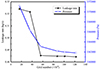 |
Fig. 2 The grid-independence analysis. |
3.2 Model validation
To verify whether the constructed model can be employed for subsequent simulation, the pipeline with a diameter of 42 mm is simulated for the leakage behaviour of nature gas based on the experiment according to the literature [24]. The leakage hole diameter is set to 3 mm and 4 mm. Meanwhile, a comparative analysis is conducted between the simulated results and the experimental results from the literature. Figure 3 shows the results of the error analysis. It can be found that the error is less than 15% between the simulated results and the experimental results. Its error may arise from environmental factors such as temperature, humidity, and wind speed, which are not considered in the model. Additionally, it could be due to the simplification of the model, such as assuming steady-state flow and neglecting variations in leakage hole geometry. Therefore, the leakage behaviour of HBNG can be predicted by employing the constructed model since the error is within the allowable range.
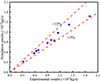 |
Fig. 3 The error analysis of the simulated results and the experimental results in the literature. |
4 Results and discussion
4.1 Influence of operating parameters
4.1.1 Hydrogen blending ratio
The different properties of hydrogen and methane indicate that hydrogen incorporation may impact gas leakage in natural gas pipelines [28]. In order to investigate whether the hydrogen blending ratio has an impact on the leakage rate, the process of gas leakage is simulated under various operating pressures. The conditions are as follows: leakage hole diameter do = 10 mm, wall thickness of pipeline δ = 9.5 mm, pipeline diameter D = 200 mm, and hydrogen blending ratio η = 0–100%. Figure 4 shows the variation results of the leakage rate under different hydrogen blending ratios. It can be found that the leakage rate decreases in direct relation to the hydrogen blending ratio when the operating pressure remains constant. The leakage rate exhibits a decrease from 1.00 kg/s to 0.33 kg/s when the hydrogen blending ratio is elevated from 0 to 100%, with the operating pressure remaining 8 MPa. This is because the low density and rapid diffusion characteristics of hydrogen lead to a decrease in the density of the mixed gas, thereby reducing the leakage rate [29, 30].
 |
Fig. 4 The variation results of leakage rate under different hydrogen blending ratios. |
4.1.2 Operating pressure
The operating pressure has a significant impact on the characteristics of gas in the pipeline. In order to investigate whether the operating pressure affects the leakage rate, the leakage process is simulated when η = 10%, 20%, and 100%, do = 10 mm and 20 mm, δ = 9.5 mm, D = 200 mm and po = 1 MPa–8 MPa. Figure 5 shows the variation results of the leakage rate under different operating pressures. It can be found that the leakage rate is a linear function of operating pressure and increases with that. The leakage rate exhibits an increase from 0.12 kg/s to 0.94 kg/s when the operating pressure is elevated from 1 MPa to 8 MPa, with the hydrogen blending ratio remaining at 10%. This is because the pressure differential becomes large between the interior and exterior of the pipeline and the gas inside the pipeline is subjected to greater thrust force as the operating pressure increases. Therefore, the leakage rate increase is linear in proportion to the increase in operating pressure.
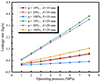 |
Fig. 5 The variation results of leakage rate under different operating pressures. |
4.2 Influence of structural parameters
4.2.1 Leakage hole diameter
The size of the leak hole directly determines the flow area of fluid through the hole and further affects the leakage rate. The leakage process for HBNG is simulated and analysed to investigate whether the leakage hole diameter affects the leakage rate. The conditions are as follows: η = 10–20%, po = 6–8 MPa, do = 0–20 mm, D = 200 mm and δ = 9.5 mm. Figure 6 shows the variation results of the leakage rate under different leakage hole diameters. It can be found that the leakage rate increases in a quadratic relationship with an increase in the leakage hole diameter. The leakage rate exhibits an increase from 0.24 kg/s to 3.83 kg/s when the leakage hole diameter is elevated from 5 mm to 20 mm, with the operating pressure remaining at 8 MPa and the hydrogen blending ratio at 10%. This is because the larger flow area through the leak hole reduces the flow resistance and redistributes the flow rates between the leak hole and the pipeline outlet. Therefore, the leakage rate is a second-order function of the leakage hole diameter. It can be found from the above that even a small increase in leak hole diameter can lead to a significant rise in leakage rate, posing serious safety, environmental, and economic risks. For HBNG pipelines, the low density and high diffusivity of hydrogen further exacerbate these risks, making it essential to implement strict leak detection and prevention measures. By monitoring and minimizing leak hole size, pipeline operators can reduce gas losses, prevent potential hazards such as fires or explosions, and ensure the safe and efficient operation of hydrogen-blended natural gas systems.
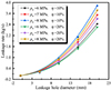 |
Fig. 6 The variation results of leakage rate under different leakage hole diameters. |
4.2.2 Pipeline diameter
When the flow rate is constant in the pipeline, the pipeline diameter will affect gas velocity. In order to investigate whether the pipeline diameter affects the leakage rate, the cases are simulated when η = 0–100%, po = 4 MPa, do = 10 mm, D = 100–400 mm, and δ = 9.5 mm. Figure 7 shows the variation results of the leakage rate under different pipeline diameters. It can be found that no matter what the pipeline diameter is, the influence of pipeline diameter is very small on the leakage rate under the same other conditions. When the hydrogen blending ratio is constant, the leakage rate with the pipeline diameter of 200 mm is slightly less than that with the pipeline diameters of 100 mm, 150 mm, and 400 mm. The influence of pipeline diameter is smaller on the leakage rate as the hydrogen blending ratio increases. Therefore, from the overall numerical point of view, the pipeline diameter has little effect on the leakage rate.
 |
Fig. 7 The variation results of leakage rate under different pipeline diameters. |
4.2.3 Wall thickness
To investigate whether the wall thickness affects the leakage rate of HBNG, four pipeline wall thicknesses are adopted according to the design of natural gas pipelines. Meanwhile, the variation of leakage rate with wall thickness is simulated under different operating pressures and hydrogen blending ratios in this section. Figure 8 shows the variation results of the leakage rate under different wall thicknesses. It can be found that when the wall thickness does not exceed 6.3 mm, the leakage rate exhibits a slight decrease as the wall thickness increases. There is no obvious change in the variation trend of leakage rate under different operating pressures and hydrogen blending ratios when the pipeline wall thickness exceeds 6.3 mm. This is because the inner diameter of the pipeline becomes relatively small as the wall thickness increases. Therefore, the wall thickness affects on the leakage rate to an extent.
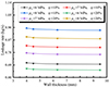 |
Fig. 8 The variation results of leakage rate under different wall thicknesses. |
4.3 Sensitivity of the leakage rate for various factors
Through the above analysis, it can be found that the hydrogen blending ratio, operating pressure, leakage hole diameter, pipeline diameter, and wall thickness have an impact on the leakage rate, but the sensitivity of the leakage rate is not known for various factors. The orthogonal design method is used to explore the influence degree of various factors on the leakage rate of HBNG in this section. The orthogonal design method is a kind of analysis method to study multi-factor and multi-level, which is mainly used to evaluate the influence of multiple variables on a certain result. According to the above simulation, five factors and three levels are considered in the orthogonal design to determine the sensitivity of the leakage rate for each factor. Table 2 shows the list of levels and factors.
The list of levels and factors.
The simulation is carried out according to the orthogonal table of L18 (35). Table 3 shows the results of the leakage rate under different simulation conditions.
The results of leakage rate under different simulation conditions.
The sensitivity of the leakage rate for various factors is judged through the range analysis of simulation results. Ki represents the average value corresponding to the level of each factor. Ri is the range value of each factor, and the expression is as follows. (11)
(11)
Based on equation (11) and Table 3, the results of range analysis are obtained by calculation, as shown in Table 4. It can be found that the range values of each factor are ranked as follows: leakage hole diameter > hydrogen blending ratio > operating pressure > wall thickness > pipeline diameter. The leakage hole diameter and pipeline diameter have the greatest and smallest effects on the leakage rate.
The results of range analysis.
In the variance analysis, F is used to test the significant effect of each factor, and the expression is as follows: (12)
(12)
Where MSSi is the mean square of each factor, and MSSe is the mean square of error. The mean square MSSi is expressed as. (13)
(13)
Where dfi is the freedom degree of each factor, and SSi is the quadratic sum of each factor. (14)
(14)
Where SSe, SSA, SSB, SSC, SSD, and SSE are the quadratic sum of leakage rate caused by error, hydrogen blending ratio, operating pressure, leakage hole diameter, pipeline diameter and wall thickness, respectively. The larger the SSi value is, the greater the impact of the corresponding factors is on the leakage rate.
Table 5 shows the results of the variance analysis. When the factor corresponding to P is less than 0.01, this factor has an extremely significant impact on the results and is denoted as “**”. When the factor corresponding to P is between 0.01 and 0.05, it has a significant impact on the results and writes “*”. When the factor corresponding to P is between 0.05 and 0.10 and more than 0.10, it has a certain extent and little effect on the results, respectively. It can be found from Table 5 that the leakage hole diameter, hydrogen blending ratio, and operating pressure have an extremely significant effect, a significant effect and to a certain extent effect on the leakage rate, respectively. The pipeline diameter and wall thickness are not significant in the leakage rate. The results of variance analysis are consistent with the results of range analysis. From a physical standpoint, the leakage hole diameter directly determines the flow area of fluid, which strongly influences the mass flow rate according to fluid dynamics principles. The hydrogen blending ratio influences the leakage behaviour by altering the physical properties of the gas mixture, such as density and viscosity. Additionally, higher operating pressure increases the pressure difference across the hole, thereby enhancing the driving force for gas leakage. In contrast, the pipeline diameter and wall thickness have little influence on the leakage rate as the flow is primarily governed by local conditions around the leakage hole rather than the global pipeline geometry.
The results of variance analysis.
4.4 New leakage model for HBNG
The different leakage models have been proposed in the literature for natural gas in low-pressure and medium-pressure overhead pipelines, as shown in Table 6. It can be found that the models do not take into account blending a proportion of hydrogen and high pressure. The hydrogen blending ratio and pressure have a significant effect on the leakage rate from the above analysis.
The leakage model for the overhead pipeline in the references.
In order to determine the suitability of existing models in the references for HBNG, the simulated values are analyzed in comparison with values calculated by models in the literature. Figure 9 shows the error analysis for the traditional model in the reference. It can be found that the correlations of Ebrahimi-Moghadam et al. [22, 26] and Hou (CD = 0.6) [21] have an appreciable deviation from simulation values and the maximum error is more than 20%. The correlation calculation values of Hou (CD = 1.0) and Montiel are consistent with the simulation values and their errors are mostly within 15%. This may be because the CD in Hou’s model is related to the geometry of the leak hole. When CD = 1.0, the leakage hole is circular. Hou’s model adds a compression factor to reduce the difference between real gas and ideal gas, but other models are assumed to be ideal gases. Therefore, the correlations of Hou (CD = 1.0) and Montiel are more effective in calculating the leakage rate.
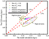 |
Fig. 9 The error analysis for the traditional model in the reference. |
In order to further analyze the factors that lead to the error of each correlation, the simulated values are compared with the values calculated by the existing models under different operating and structural parameters. Figures. 10a–10c show the comparisons between CFD values in this paper and calculated values based on Table 6 under hydrogen blending ratios, operating pressures and leakage hole diameters, respectively. It can be found that there is a significant deviation between leakage rates calculated by each model under the same conditions. The hydrogen blending ratio exerts the greatest influence on the deviation of the leakage rate calculated by each model.
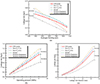 |
Fig. 10 The comparisons between CFD values in this paper and calculated values based on Table 6. a) At different hydrogen blending ratios; b) At different operating pressures; c) At different leakage hole diameters. |
In order to obtain a more accurate leakage model for HBNG, A new prediction model of leakage rate is proposed in accordance with the simulated values. The proposed prediction model is expressed as follows. (15)
(15)
Where Q0 is the leakage rate of HBNG, η is the hydrogen blending ratio, po is the operating pressure, do is the leakage hole diameter. The proposed prediction model is applicable for high-pressure HBNG overhead pipelines with operating pressures of 1–8 MPa, leakage hole diameters below 20 mm, and hydrogen blending ratios of 0–100%.
Figure 11 is the error analysis of the simulated values and the predicted values of the new prediction model. It can be found that the leakage rate predicted by equation (15) is in good agreement with simulated values, and the predicted error is within 5% between the simulated values and the predicted values of the new model. It shows that the prediction model is reliable for the leakage rate. The new prediction can provide theoretical guidance for the leakage of high-pressure pipelines and prediction in engineering.
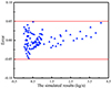 |
Fig. 11 The error analysis of the simulated values and the values predicted by the new model. |
5 Conclusion
In this paper, a mathematical-physical model is established for HBNG leakage based on species transport and a real-gas model. Meanwhile, the influence of different operating and structural parameters is analyzed on the leakage rate of HBNG, and the orthogonal design is used in this simulation to analyse the effect of different factors on the leakage rate. A new prediction model of the leakage rate is proposed according to the simulation values. The following conclusions can be drawn:
-
For operating parameters, the leakage rate decreases with an increase in the hydrogen blending ratio. This is because the low density and rapid diffusion characteristics of hydrogen lead to a decrease in the density of the mixed gas, thereby reducing the leakage rate. The leakage rate increases linearly with increasing operating pressure. This is because when the operating pressure increases, the pressure differential increases between the interior and exterior of the pipeline.
-
For structural parameters, the leakage rate increases in a quadratic relationship with an increase in leakage hole diameter. When the wall thickness does not exceed 6.3 mm, it has little effect on the leakage rate. When pipeline wall thickness exceeds 6.3 mm, there is no significant change in the variation trend of the leakage rate under different conditions.
-
The sensitivity of leakage rate for various factors ranks as follows: leakage hole diameter > hydrogen blending ratio > operating pressure > wall thickness > pipeline diameter. It should be pointed out that the wall thickness and pipeline diameter have very little effect on the leakage rate.
-
The new leakage prediction model is highly accurate with a prediction deviation of less than 5%, which can be used to predict the leakage rate of HBNG.
The above research results can be used as guidance for risk assessment and prevention of accidents for HBNG in high-pressure overhead pipelines. However, the leakage characteristics of HBNG are only analysed in a steady state. In the future, it is suggested to investigate unsteady leakage and diffusion characteristics in HBNG to further determine the leakage behaviour.
Funding
This works was supported by the National Natural Science Foundation [grant number 52368071 and 52478515] and the Jiangxi Province Innovation Leading Talent Project [grant number jxsq2023101064 and jxsq2023102132].
Conflicts of interest
The authors declare that we have no financial or personal relationships with other people or organizations that can inappropriately influence our work.
Data availability statement
No data was used for the research described in the article.
Author contribution statement
Ting Zhang: Software, Validation, Investigation. Guohua Xiong: Conceptualization, Formal analysis, Investigation, Methodology, Hongqiang Ma: Conceptualization, Formal analysis, Investigation, Methodology, Project administration, Supervision, Writing – original draft. Yue Zeng: Writing – review & editing, Supervision. Huilun Kang: Writing – review & editing, Supervision. Jing Wu: Writing – review & editing, Supervision. Xiaosong Cheng: Writing – review & editing, Supervision.
References
- Ishaq H., Dincer I. (2021) Comparative assessment of renewable energy-based hydrogen production methods, Renew. Sustain. Energy Rev. 135, 110192. [Google Scholar]
- Huang J., Lu D., Huang X., Hu Z., Liu L., Lin C., Jing R., Xie C., Brandon N., Zheng X., Zhao Y. (2024) Is China ready for a hydrogen economy? Feasibility analysis of hydrogen energy in the Chinese transportation sector, Renew. Energy 223, 119964. [Google Scholar]
- Ma H., Zhong Y., Wang J., Xie Y., Ding R., Kang R., Zeng Y. (2024) Method for identifying the leakage of buried natural gas pipeline by soil vibration signals, J. Nat Gas Sci.Eng 132, 205487. [Google Scholar]
- Tu R., Liu C., Shao Q., Liao Q., Qiu R., Liang Y. (2024) Pipeline sharing: optimal design of downstream green ammonia supply systems integrating with multi-product pipelines, Renew. Energy 223, 120024. [Google Scholar]
- Yang F., Wang T., Deng X., Dang J., Huang Z., Hu S., Li Y., Ouyang M. (2021) Review on hydrogen safety issues: incident statistics, hydrogen diffusion, and detonation process, Int. J. Hydrogen Energy 46, 31467–31488. [Google Scholar]
- Fúnez Guerra C., Reyes-Bozo L., Vyhmeister E., Jaén Caparrós M., Salazar J.L., Clemente-Jul C. (2020) Technical-economic analysis for a green ammonia production plant in Chile and its subsequent transport to Japan, Renew. Energy 157, 404–414. [Google Scholar]
- Ma H., Wang S., Wang J., Xie Y., Zhong P., Cai W., Min K., Luo X. (2023) Investigation on strength and fracture mechanism of aluminum plate-fin structures at cryogenic temperature, Eng. Fail. Anal, 152, 107512. [Google Scholar]
- Ma H.,Ding R., He B., Liu Q., Xu G., Qian S., Fu H. (2023) Numerical investigation of the strain characteristics of a natural gas transportation pipeline crossing tunnel, Transport. Res. Rec. 2677, 51–61. [Google Scholar]
- Carlson E.L., Pickford K., Nyga-Łukaszewska H. (2023) Green hydrogen and an evolving concept of energy security: challenges and comparisons, Renew. Energy 219, 119410. [Google Scholar]
- Hafsi Z., Elaoud S., Mishra M. (2019) A computational modelling of natural gas flow in looped network: effect of upstream hydrogen injection on the structural integrity of gas pipelines, J. Nat. Gas Sci. Eng. 64, 107–117. [CrossRef] [Google Scholar]
- Kostowski W.J., Skorek J. (2012) Real gas flow simulation in damaged distribution pipelines, Energy 45, 481–488. [Google Scholar]
- Yan Y., Dong X., Li J. (2015) Experimental study of methane diffusion in soil for an underground gas pipe leak, J. Nat. Gas Sci. Eng. 27, 82–89. [Google Scholar]
- Yuan F., Zeng Y., Luo R., Khoo B.C. (2020) Numerical and experimental study on the generation and propagation of negative wave in high-pressure gas pipeline leakage, J. Loss Prev. Process Ind. 65, 104129. [Google Scholar]
- Montiel H., Vilchez J., Casal J., Arnaldos J. (1998) Mathematical modelling of accidental gas releases, J. Hazard. Mater. 59, 211–233. [Google Scholar]
- Wang D.W., Huo C.Y., Gao H.L. (2008) Simplified calculation method of gas leakage rate of long-distance pipeline, Nat. Gas Ind. 1, 116–118+174–175. [Google Scholar]
- Arnaldos J., Casal J., Montiel H., Sánchez-Carricondo M., Vílchez J.A. (1998) Design of a computer tool for the evaluation of the consequences of accidental natural gas releases in distribution pipes, J. Loss Prev. Process Ind. 11, 135–148. [Google Scholar]
- Hou Z., Yuan X. (2021) Leakage locating and sampling optimization of small-rate leakage on medium-and-low-pressure unground natural gas pipelines, J. Nat. Gas Sci. Eng. 94, 104112. [Google Scholar]
- He G., Liang Y., Li Y., Wu M., Sun L., Xie C., Li F. (2017) A method for simulating the entire leaking process and calculating the liquid leakage volume of a damaged pressurized pipeline, J. Hazard. Mater. 332, 19–32. [Google Scholar]
- Jo Y. (2003) A simple model for the release rate of hazardous gas from a hole on high-pressure pipelines, J. Hazard. Mater. 97, 31–46. [Google Scholar]
- Moloudi R., Abolfazli Esfahani J. (2014) Modeling of gas release following pipeline rupture: Proposing non-dimensional correlation, J. Loss Prev. Process Ind. 32, 207–217. [Google Scholar]
- Hou Q., Yang D., Li X., Xiao G., Ho S.C.M. (2020) Modified leakage rate calculation models of natural gas pipelines, Math. Probl. Eng. 2020, 1–10. [Google Scholar]
- Nagase Y., Sugiyama Y., Kubota S., Saburi T., Matsuo A. (2019) Prediction model of the flow properties inside a tube during hydrogen leakage, J. Loss Prev. Process Ind. 62, 103955. [Google Scholar]
- Wang L., Chen J., Ma T., Ma R., Bao Y., Fan Z. (2024) Numerical study of leakage characteristics of hydrogen-blended natural gas in buried pipelines, Int. J. Hydrogen Energy 49, 1166–1179. [Google Scholar]
- Liang J. (2019) Research on leakage amount estimation and diffusion characteristics for buried gas pipeline, PhD thesis, China University of Petroleum (East China). [Google Scholar]
- Yuan F., Zeng Y., Khoo B.C. (2022) A new real-gas model to characterize and predict gas leakage for high-pressure gas pipeline, J. Loss Prev. Process Ind. 74, 104650. [Google Scholar]
- Zhou X., Li K., Tu R., Yi J., Xie Q., Jiang X. (2016) A modelling study of the multiphase leakage flow from pressurised CO2 pipeline, J. Hazard. Mater. 306, 286–294. [Google Scholar]
- Ebrahimi-Moghadam A., Farzaneh-Gord M., Deymi-Dashtebayaz M. (2016) Correlations for estimating natural gas leakage from above-ground and buried urban distribution pipelines, J. Nat. Gas Sci. Eng. 34, 185–196. [Google Scholar]
- Uilhoorn F.E. (2013) A comparison between PSRK and GERG-2004 equation of state for simulation of non-isothermal compressible natural gases mixed with hydrogen in pipelines, Arch. Min. Sci. 58, 579–590. [Google Scholar]
- Zhu J., Pan J., Zhang Y., Li Y., Li H., Feng H., Chen D., Kou Y., Yang R. (2023) Leakage and diffusion behavior of a buried pipeline of hydrogen-blended natural gas, Int. J. Hydrogen Energy 48, 11592–11610. [CrossRef] [Google Scholar]
- Zhou C., Yang Z., Chen G., Zhang Q., Yang Y. (2022) Study on leakage and explosion consequence for hydrogen blended natural gas in urban distribution networks, Int. J. Hydrogen Energy 47, 27096–27115. [CrossRef] [Google Scholar]
- Ebrahimi-Moghadam A., Farzaneh-Gord M., Arabkoohsar A., Moghadam A.J. (2018) CFD analysis of natural gas emission from damaged pipelines: Correlation development for leakage estimation, J. Clean. Prod. 199, 257–271. [Google Scholar]
All Tables
All Figures
|
Fig. 1 The three-dimensional model of HBNG leakage. a) The schematic diagram; b) The pipeline of leakage. |
| In the text | |
|
Fig. 2 The grid-independence analysis. |
| In the text | |
|
Fig. 3 The error analysis of the simulated results and the experimental results in the literature. |
| In the text | |
|
Fig. 4 The variation results of leakage rate under different hydrogen blending ratios. |
| In the text | |
|
Fig. 5 The variation results of leakage rate under different operating pressures. |
| In the text | |
|
Fig. 6 The variation results of leakage rate under different leakage hole diameters. |
| In the text | |
|
Fig. 7 The variation results of leakage rate under different pipeline diameters. |
| In the text | |
|
Fig. 8 The variation results of leakage rate under different wall thicknesses. |
| In the text | |
|
Fig. 9 The error analysis for the traditional model in the reference. |
| In the text | |
|
Fig. 10 The comparisons between CFD values in this paper and calculated values based on Table 6. a) At different hydrogen blending ratios; b) At different operating pressures; c) At different leakage hole diameters. |
| In the text | |
|
Fig. 11 The error analysis of the simulated values and the values predicted by the new model. |
| In the text | |
Current usage metrics show cumulative count of Article Views (full-text article views including HTML views, PDF and ePub downloads, according to the available data) and Abstracts Views on Vision4Press platform.
Data correspond to usage on the plateform after 2015. The current usage metrics is available 48-96 hours after online publication and is updated daily on week days.
Initial download of the metrics may take a while.