© The Author(s), published by EDP Sciences, 2026

1 Introduction

Nowadays, industry is shifting toward advanced and sophisticated electric drive systems, increasingly adopting multi-machine, multi-converter configurations to meet growing and specific industrial needs [1, 2]. In the past, drive systems were relatively simple, typically consisting of an electric motor connected to a frequency converter. While this setup was effective for basic speed and torque control in certain applications, it was often bulky in terms of volume [3]. In this context, Multi-Drive Web Winding System (MDWWS) have emerged. These systems consist of multiple electric motors, each driven by a voltage inverter, all connected to a common DC bus [2]. Multi-Motor System has become widespread in industries that naturally require distributed actuators, such as the paper, plastic [1], textile [4], and metalworking industries [5], among others. They are specifically designed to meet the needs of these sectors in terms of speed control, mechanical tension, torque regulation, and the handling of rolled/unrolled materials.

The main objective of the control system in web handling processes is to maintain continuous production by preventing web breaks, folds, or damage. Significant fluctuations in speed or mechanical tension can cause premature wear or even complete loss of the web. To address this, the control system must ensure accurate regulation of both speed and tension, with effective decoupling to avoid undesirable interactions between them. Additionally, it must demonstrate robustness to mechanical variations, such as changes in the inertia of the unwinding/rewinding units and in the web’s Young’s modulus. Fulfilling these requirements is crucial to maintaining the quality and reliability of the industrial process.

Many industrial web transport systems have employed decentralized PI controllers [6]. A comprehensive review of web tension control challenges can be found in [7]. Alternative control approaches have also been explored, including fuzzy logic [8, 9], neural networks [10], optimal control [11], nonlinear sliding mode control [12, 13], Active Disturbance Rejection Control (ADRC) [14, 15], and robust control methods [16]. Robust feedback control based on Lyapunov theory [17] and multivariable H_∞ controllers have also been proposed for web handling systems [18]. Among the most prominent nonlinear control design techniques is the Backstepping approach. Adaptive Backstepping control aims to achieve precise coordination between motors while compensating for load variations and external disturbances. This nonlinear strategy is grounded in feedback principles, allowing dynamic adjustment of system parameters to ensure optimal performance [19].

In this study, our contribution focuses on improving the system’s robustness to parametric variations in the Young’s modulus and the total inertias of the winder and unwinder by designing a nonlinear controller based on the integral Backstepping approach. This method is intended to simultaneously control the web’s scrolling speed and mechanical tension within the system under study, as shown in Figure 1.

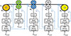Figure 1 Backstepping control structure applied to the MDWWS.

The validation of control strategies within a Model-Based Design (MBD) framework is carried out using Processor-in-the-Loop (PIL) simulation to assess the performance of controllers on a MDWWS model [20, 21]. This hybrid simulation technique is especially effective for rapid prototyping. In this setup, the system model runs in Simulink, while control and observation algorithms are executed in real time on the TMDSCNCD28379D DSP board (see Fig. 2). This configuration offers a realistic and efficient environment to evaluate control performance under near-real-world conditions before implementation on the physical system.

Figure 2 Operation of the hybrid Processor-in-the-Loop (PIL) platform.

The structure of this paper is organized to provide a clear and progressive understanding of the proposed approach. Section 2 presents the dynamic modeling of the web winding system, with particular emphasis on the mechanical coupling between the multiple motors and the web material. In Section 3, the design and formulation of the nonlinear control strategy based on the integral Backstepping technique are detailed, targeting precise regulation of both mechanical tension and transport speed. Section 4 showcases the simulation results conducted in MATLAB/Simulink, including a Processor-in-the-Loop (PIL) implementation, to evaluate the controller’s performance under various operating scenarios. Lastly, Section 5 summarizes the key findings and concludes the study, highlighting potential avenues for future work.

2 Mathematical Modeling of the Web Winding System

Figure 3 illustrates a basic multi-motor web transport setup, typically found in winder systems, featuring two motors: M₁ for unwinding and M₂ for winding. The modeling of these systems is based on three core principles: Hooke’s law, Coulomb’s law, and the law of mass conservation, which together enable the calculation of web tension between the two rolls [22–24].

Figure 3 Web tension in roll handling.

Equation (1) defines the web tension T₂ as a function of the web length L and the linear speeds of motors V₁ and V₂.$$L\frac{\mathrm{d}{T}_2}{\mathrm{d}t}\cong \mathrm{ES}\left(V_2-V_1\right)+T_1{V}_1-T_2\left(2V_1-V_2\right).$$(1)

The Multi-Drive Web Winding System under analysis comprises five motors, and its dynamic behavior, specifically motor speeds and web tension, is characterized by the following set of equations: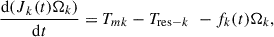$$\frac{\mathrm{d}{(J}_k\left(t\right){\Omega }_k)}{\mathrm{d}t}=T_{\mathrm{mk}}-T_{\mathrm{res}-k} -f_k\left(t\right){\Omega }_k,$$(2) $$L_{k+1}\frac{\mathrm{d}{T}_{k+1}}{\mathrm{d}t}=\mathrm{ES}\left(V_{k+1}-V_k\right)+T_k{V}_k-T_{k+1}{V}_{k+1}.$$(3)

For k = 1 to 5, the expressions V_k = R_k Ω_k and T_res-k = R_k (T_k − T_k+1) represent the linear web speed and the load torque disturbance, respectively, where Ω_k is the rotational speed and R_k denotes the roll radius.

By reformulating equations (2) and (3), the state-space representation of the Multi-Drive Web Winding System is obtained as follows:$$\dot{X}=\mathrm{AS}-B-\mathrm{CX},$$(4)where:$$S=\left[\begin{array}{c}\begin{array}{c}{V}_2\\ V_3\\ V_4\\ V_5\end{array}\\ T_{m1}\\ T_{m2}\\ T_{m3}\\ T_{m4}\\ T_{m5}\end{array}\right],\hspace{1em}X=\left[\begin{array}{c}\begin{array}{c}{T}_2\\ T_3\\ T_4\\ T_5\end{array}\\ {\mathrm{\Omega }}_1\\ {\mathrm{\Omega }}_2\\ {\mathrm{\Omega }}_3\\ {\mathrm{\Omega }}_4\\ {\mathrm{\Omega }}_5\end{array}\right],$$ $$A=\left[\begin{array}{ccccccccc}\frac{\mathrm{ES}}{L_2}& 0& 0& 0& 0& 0& 0& 0& 0\\ 0& \frac{\mathrm{ES}}{L_2}& 0& 0& 0& 0& 0& 0& 0\\ 0& 0& \frac{\mathrm{ES}}{L_2}& 0& 0& 0& 0& 0& 0\\ 0& 0& 0& \frac{\mathrm{ES}}{L_2}& 0& 0& 0& 0& 0\\ 0& 0& 0& 0& \frac{1}{J_1}& 0& 0& 0& 0\\ 0& 0& 0& 0& 0& \frac{1}{J_2}& 0& 0& 0\\ 0& 0& 0& 0& 0& 0& \frac{1}{J_3}& 0& 0\\ 0& 0& 0& 0& 0& 0& 0& \frac{1}{J_4}& 0\\ 0& 0& 0& 0& 0& 0& 0& 0& \frac{1}{J_5}\end{array}\right] ,$$ $$B=\left[\begin{array}{c}\begin{array}{c}{V}_1(\mathrm{ES}-T_1)\\ V_2(\mathrm{ES}-T_2)\\ V_3(\mathrm{ES}-T_3)\\ V_4(\mathrm{ES}-T_4)\end{array}\\ \frac{R_1}{J_1}(T_1-T_2)\\ \frac{R_2}{J_2}(T_2-T_3)\\ \frac{R_3}{J_3}(T_3-T_4)\\ \frac{R_4}{J_4}(T_4-T_5)\\ \frac{R_5}{J_5}(T_5-T_S)\end{array}\right],$$ $$C=\left[\begin{array}{ccccccccc}{V}_2& 0& 0& 0& 0& 0& 0& 0& 0\\ 0& V_3& 0& 0& 0& 0& 0& 0& 0\\ 0& 0& V_4& 0& 0& 0& 0& 0& 0\\ 0& 0& 0& V_5& 0& 0& 0& 0& 0\\ 0& 0& 0& 0& \frac{f_1}{J_1}& 0& 0& 0& 0\\ 0& 0& 0& 0& 0& \frac{f_2}{J_2}& 0& 0& 0\\ 0& 0& 0& 0& 0& 0& \frac{f_3}{J_3}& 0& 0\\ 0& 0& 0& 0& 0& 0& 0& \frac{f_4}{J_4}& 0\\ 0& 0& 0& 0& 0& 0& 0& 0& \frac{f_5}{J_5}\end{array}\right].$$

Matrices A and C are square and diagonal matrices of size n × n. The matrix B ∈ R ⁿ represents the control input. The state vector X ∈ R ⁿ characterizes the system dynamics, while the vector S ∈ R ⁿ includes the torque and speed components of each motor.

3 Design of the control law for the MDWWS using Integral Backstepping

The primary objective of applying the Backstepping method is to achieve asymptotic convergence of the vector γ towards a bounded reference vector γ_ref, where$X=\frac{\mathrm{d}\gamma }{\mathrm{d}t}$. The set of internal signals is utilized within the context of the closed-loop system [25–27].

Initially, the first step consists of defining the error between γ and γ_ref.$${\epsilon }_{\gamma }={\gamma }_{\mathrm{ref}}- \gamma .$$(5)

The dynamics of which can be expressed as follows:$${\dot{\epsilon }}_{\gamma }={\dot{\gamma }}_{\mathrm{ref}}-X.$$(6)

This definition outlines our control objective, which is to drive the error ε_γ to asymptotically converge to zero. This goal will be accomplished through our incremental design approach. In fact, the convergence rate of the error ε_γ can be controlled by incorporating the integration of ε_γ as follows:$${\epsilon }_I=\underset{0}{\overset{t}{\int }}{\epsilon }_{\gamma }\left(\tau \right)\mathrm{d}\tau .$$(7)

We will now extend the system to the subsystem $($∆₁) (8). The state representation then becomes:$${∆}_1\{\begin{array}{c}{\dot{\epsilon }}_i= {\epsilon }_{\gamma }\\ {\dot{\epsilon }}_{\gamma }={\dot{\gamma }}_{\mathrm{ref}}-X\end{array}.$$(8)

The first Lyapunov function is chosen in the following format: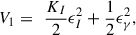$$V_1= \frac{K_I}{2}{\epsilon }_I^2+\frac{1}{2}{\epsilon }_{\gamma }^2,$$(9)where K_I is a positive constant that adjusts the value of the integral to be incorporated into the system dynamics.

We now choose the virtual control law X so that the derivative of V₁, denoted $\dot{V_1}$, is less than or equal to 0. According to Lyapunov stability theory, it is known that such a control law stabilizes the first subsystem (∆₁).

We now define the virtual control law X such that the derivative of V₁, denoted $\dot{V_1}$, is less than or equal to zero. According to Lyapunov stability theory, this control law ensures the stabilization of the first subsystem (∆₁).

Now, considering:$$X=K_{\gamma }{\epsilon }_{\gamma }+{\dot{\gamma }}_{\mathrm{ref}}+K_I{\epsilon }_I.$$(10)

The derivative of the Lyapunov control function is then given by:$$\dot{V_1}=-K_{\gamma }{\epsilon }_{\gamma }^2.$$(11)

Now, we can consider X in (10) as a reference (X_ref) for the next design step.

Next, we proceed to the following step, which focuses on ensuring that the signals X track their reference X_ref. To accomplish this, we can derive the dynamics of the error between the vectors X and X_ref as follows:$${\dot{\epsilon }}_{V-T}=K_{\gamma }\left({\dot{\gamma }}_{\mathrm{ref}}-X\right)+{\ddot{\gamma }}_{\mathrm{ref}}+K_I{\epsilon }_{\gamma }-\mathrm{AS}+B+\mathrm{CX},$$(12)where ε_V-T corresponds to X_ref − X, representing the error vector of the motor speeds and the tensions in the web.

Now, let’s extend once again the last subsystem (∆₂), which is described by the following equations:$${∆}_2\{\begin{array}{c}{\dot{\epsilon }}_i= {\epsilon }_{\gamma }\\ {\dot{\epsilon }}_{\gamma }={-K}_p{\epsilon }_{\gamma }{-K}_I{\epsilon }_I+{\epsilon }_{V-T}\\ {\dot{\epsilon }}_{V-T}=K_{\gamma }\left({\dot{\gamma }}_{\mathrm{ref}}-X\right)+{\ddot{\gamma }}_{\mathrm{ref}}+K_I{\epsilon }_{\gamma }-\mathrm{AS}\\ +B+\mathrm{CX}\end{array}.$$(13)

By introducing S as a virtual control input, the overall system can be stabilized using the Lyapunov function V₂.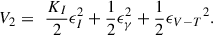$$V_2= \frac{K_I}{2}{\epsilon }_I^2+\frac{1}{2}{\epsilon }_{\gamma }^2+\frac{1}{2}{{\epsilon }_{V-T}}^2.$$(14)

Whose time derivative of V₂ is:$$\dot{V_2}=-K_{\gamma }{\epsilon }_{\gamma }^2+{\epsilon }_{V-T}\left\{{\epsilon }_{\gamma }+K_{\gamma }\left(-K_{\gamma }{\epsilon }_{\gamma }-K_I{\epsilon }_I+{\epsilon }_{V-T}\right)+{\ddot{\gamma }}_{\mathrm{ref}}+K_I{\epsilon }_{\gamma }-\mathrm{AS}+B+\mathrm{CX} \right\}.$$(15)

We select the virtual stabilization control law to ensure that $\dot{V_2}$ is negative. Assuming all parameters in the matrices A, B, and C are known, the control law S that stabilizes the entire system is as follows:$$\begin{array}{c}S =A^{-1}\left\{K_V{\epsilon }_{V-T}+{\epsilon }_{\gamma }+K_{\gamma }\left(-K_{\gamma }{\epsilon }_{\gamma }-K_I{\epsilon }_I+{\epsilon }_{V-T}\right)+{\ddot{\gamma }}_{\mathrm{ref}}+K_I{\epsilon }_{\gamma }+B+\mathrm{CX}\right\}\\ ={ A}^{-1}\left\{\left(1-{K_{\gamma }}^2+K_I\right){\epsilon }_{\gamma }+\left(K_{\gamma }+K_V\right){\epsilon }_{V-T}-K_{\gamma }{K}_I{\epsilon }_I+{\ddot{\gamma }}_{\mathrm{ref}}+B+\mathrm{CX}\right\}\end{array}.$$(16)

The time derivative of the Lyapunov function V₂ becomes: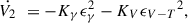$$\dot{V_2} =-K_{\gamma }{\epsilon }_{\gamma }^2-K_V{{\epsilon }_{V-T}}^2,$$(17)where K_γ > 0 and K_V > 0 are tuning parameters. As a result, the virtual control law S stabilizes the last subsystem (∆₂) since the time derivative $\dot{V_2}$ is semi-negative along its trajectories, ensuring the convergence of the error ε_V-T.

Since the parameter matrices A, B, and C are unknown, we use their estimates, denoted $\widehat{A},\widehat{B}$ and $\widehat{C}$ [28]. We choose to implement an indirect adaptive control law as follows:$$U={\widehat{A}}^{-1}\left\{\left(1-K_{\gamma }^2+K_I\right){\epsilon }_{\gamma }+\left(K_{\gamma }+K_V\right){\epsilon }_{V-T}-K_{\gamma }{K}_I{\epsilon }_I+{\ddot{\gamma }}_{\mathrm{ref}}+\widehat{B}+\widehat{C}X\right\}.$$(18)

The adaptation law for the matrices is given by:$$\{\begin{array}{c}\dot{{\widehat{A}}^{-1}}={\delta }_1{\epsilon }_{V-T}\left[\begin{array}{c}\left(1-{K_{\gamma }}^2+K_I\right){\epsilon }_{\gamma }+\\ \left(K_{\gamma }+K_V\right){\epsilon }_{V-T}\\ -K_{\gamma }{K}_I{\epsilon }_I+{\ddot{\gamma }}_{\mathrm{ref}}\\ +\widehat{B}+\widehat{C}X\end{array}\right]\\ \dot{\widehat{B}}={\delta }_2{\epsilon }_{V-T}\\ \dot{\widehat{C}}={\delta }_3{\epsilon }_{V-T}X\end{array}.$$(19)

4 Validation of Backstepping Integrator Control through the PIL technique

In our PIL application, we utilize the integrated MATLAB/Simulink environment, covering the design, code generation, and PIL co-simulation with the TMDSCNCD28379D development kit for the C2000™ Delfino MCU controlCARD™. The following sections will describe the development environment, the code generation process, and the co-simulation steps.

The IBSC (Integrator Backstepping Control) discussed earlier is implemented in discrete mode within Simulink, integrated into the “IBSC_Discret” block, as shown in Figure 4. The continuous mode applies to the multi-motor system model. The two modes are separated by sample-and-hold blocks with a sampling period of T_e = 200 μs and simulation step-size adaptation blocks.

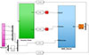Figure 4 Discrete implementation of backstepping integrator control in simulink.

After testing the setup in the Simulink simulator, the “IBSC_Discret” block is converted into a subsystem for automatic code generation in C or C⁺⁺. This generates a new block, “IBSC_PIL,” with “PIL” added in the middle of its name. This block is then integrated into the simulation environment and prepared for validation using the “Processor-In-the-Loop” (PIL) technique, as shown in Figure 5.

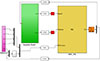Figure 5 Code and PIL block generation in simulink.

The test setup, shown in Figure 6, involves generating code based on the IBSC model, compiling it, and executing it on the TMDSCNCD28379D target. The goal is to validate the generated code by comparing its results with those from the Simulink model. In this PIL configuration, the speed and mechanical tension values calculated in Simulink are sent as inputs to the IBSC_PIL algorithm running on the F28379D DSP. The PIL block in Simulink serves as an interface, transmitting inputs to the DSP, while the control algorithm outputs are returned to the Simulink model via USB serial communication. To validate the effectiveness of the proposed integrator Backstepping control, we also implemented a control system using standard PI controllers for comparison. This comparison was performed under the following conditions:

• All parameters are perfectly known.

• The Young’s modulus E is underestimated by a factor of 2 in the controller.

• The total inertias J₁ and J₅, as perceived by the motors M₁ and M₅, respectively, are overestimated by a factor of 2.

Figure 6 Test setup for PIL co-simulation.

Reference signals for mechanical tension are applied progressively to different sections of the web, starting from the last and moving towards the first. A filtered speed ramp is then applied to the web, as shown in Figures 6 and 7. The winder system and control parameters used in the simulations are detailed in Appendix A.

Figure 7 Reference linear speed for master motor M2.

In the analysis of the results shown in Figure 8, we observe that the tensions of the last four motors (T₂, T₃, T₄, T₅) quickly converge to their setpoint values, represented by 4 N steps. Examining the results for the tensions and speeds (Figs. 9 and 10) of these motors, we find that the steady-state errors are also zero. However, oscillations appear in the mechanical tensions during the transient state. These oscillations can be attributed to the increased order of the subsystems, the use of derivatives in the controller, and the couplings between the control loops, demonstrating the challenges associated with the system’s increasing complexity.

Figure 8 Mechanical tension references.

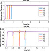Figure 9 Responses of mechanical tensions by PIL.

Figure 10 Response speeds of the five motors by PIL.

To quantitatively evaluate the controller’s performance, the Integral of Squared Error (ISE) performance index is utilized. This evaluation is conducted using both exact parameters and underestimations of E, J₁ and J₂. The ISE values, calculated over the time range [0s–1s] for tension errors ∆T₂, ∆T₃, ∆T₄, and T₅ are provided in Table 1.

The obtained results clearly demonstrate the superior robustness of the proposed Integrator Backstepping controller when subjected to variations in system parameters, particularly the inertia of the rolls and the Young’s modulus of the web. In contrast to the conventional PI controller, the IBSC consistently maintains better stability and accuracy, even under dynamic and uncertain operating conditions. This highlights its effectiveness in ensuring reliable control performance in real industrial environments.

5 Conclusion

This paper presented a robust nonlinear control strategy designed for the independent regulation of the master motor speed and mechanical tensions within a Multi-Drive Web Winding System (MDWWS). The control architecture is built upon the Integral Backstepping approach, which enables precise tracking of both speed and tension setpoints, even in the presence of significant parameter uncertainties, such as changes in the Young’s modulus and the total inertias of the winder and unwinder units. The effectiveness of the proposed controller was thoroughly validated through both simulation (modeling and control in MATLAB/Simulink) and Processor-in-the-Loop (PIL) co-simulation using the TMDSCNCD28379D DSP board. Compared to the classical PI control strategy, the proposed solution exhibited superior performance and enhanced robustness under varying conditions.

Looking ahead, future research will focus on extending the validation process to include additional frameworks such as Hardware-in-the-Loop (HIL) testing. These studies will also explore implementation across diverse digital hardware platforms, including alternative DSPs, ASICs, and FPGAs, to further assess the scalability and real-time performance of the proposed control method.

References

Appendix A: Parameters simulations.

Appendix B

Specifications of development board TMDSCNCD28379D F28379D development kit for C2000™ Delfino MCU controlCARD™ [29].

Technical specifications of the TMDSDOCK28379D board:

• CPU: C28x.

• Memory: 1MB flash.

• 24 PWM and four 16bit or 12bit ADCs, sigma delta filter modules, capture interfaces, QEP interfaces, and serial connectivity.

• On-board emulator: XDS100 USB JTAG.

All Tables

All Figures

	Figure 1 Backstepping control structure applied to the MDWWS.
In the text

	Figure 2 Operation of the hybrid Processor-in-the-Loop (PIL) platform.
In the text

	Figure 3 Web tension in roll handling.
In the text

	Figure 4 Discrete implementation of backstepping integrator control in simulink.
In the text

	Figure 5 Code and PIL block generation in simulink.
In the text

	Figure 6 Test setup for PIL co-simulation.
In the text

	Figure 7 Reference linear speed for master motor M2.
In the text

	Figure 8 Mechanical tension references.
In the text

	Figure 9 Responses of mechanical tensions by PIL.
In the text

	Figure 10 Response speeds of the five motors by PIL.
In the text

References

- Chen D., Wang M. (2006) Adaptive control of linear velocity and tension in winding system of dry plastic film laminating machine, in 2006 International Technology and Innovation Conference (ITIC 2006), Hangzhou, pp. 1919–1923.https://doi.org/10.1049/cp:20061081. [Google Scholar]
- Foti S., Testa A., De Caro S., Scimone T., Scelba G., Scarcella G. (2019) Multi-level open end windings multi-motor drives, Energies 12 (5), 5. https://doi.org/10.3390/en12050861. [Google Scholar]
- Al Sakka M., Geury T., El Baghdadi M., Dhaens M., Al Sakka M., Hegazy O. (2022) Review of fault tolerant multi-motor drive topologies for automotive applications, Energies 15, 15, 15. https://doi.org/10.3390/en15155529. [Google Scholar]
- Rawat P., Liu S., Mahesh Kumar R., Singh N.K. (2023) Numerical investigation on the high-velocity impact resistance of textile reinforced composite mesh designs inspired by spider web, J Text. Inst. 115, 1995–2010. https://doi.org/10.1080/00405000.2023.2276863. [Google Scholar]
- Kuznetsov B., Nikitina T., Bovdui I.V. (2020) Structural-parametric synthesis of rolling mills multi-motor electric drives, Electr. Eng. Electromechanics 5, 25–30. https://doi.org/10.20998/2074-272X.2020.5.04. [Google Scholar]
- Nishida T. (2013) Self-tuning PI control using adaptive PSO of a Web transport system with overlapping decentralized control, Electr. Eng. Jpn. 184, 56–65. [Google Scholar]
- Wolfermann W. (1995) Tension control of webs – A review of the problems and solutions in the present and future. Accessed: Oct. 14, 2023. [Online]. Available: https://shareok.org/handle/11244/321706. [Google Scholar]
- Ponniah G., Zubair M., Doh Y., Choi K. (2013) Fuzzy decoupling to reduce propagation of tension disturbances in roll-to-roll system, Int. J. Adv. Manuf. Technol. 71, 1–4. https://doi.org/10.1007/s00170-013-5400-4. [Google Scholar]
- Jee S., Kim S., Shin K.-H. (1999) Adaptive fuzzy control of tension variations due to the eccentric unwinding roll in multi-span web transport systems, in Proceedings of the ASME 1999 International Mechanical Engineering Congress and Exposition. Dynamic Systems and Control. Nashville, Tennessee, USA. November 14–19, The American Society of Mechanical Engineers, pp. 877–882. https://doi.org/10.1115/IMECE1999-0119. [Google Scholar]
- Wang C., Wang Y., Yang R., Lu H. (2004) Research on precision tension control system based on neural network, Ind. Electron. IEEE Trans. On 51, 381–386. https://doi.org/10.1109/TIE.2003.822096. [Google Scholar]
- Angermann A., Aicher M., Schroder D. (2000) Time-optimal tension control for processing plants with continuous moving webs, in: Proc. 35th Annual Meeting-IEEE Industry Applications Society, Rome, Rome, pp. 3505–3511. https://doi.org/10.1109/IAS.2000.882671. [Google Scholar]
- Abjadi N.R., Soltani J., Askari J., Markadeh G.R.A. (2009) Nonlinear sliding-mode control of a multi-motor web-winding system without tension sensor, IET Control Theory Amp. Appl. 3, 4, 419–427. https://doi.org/10.1049/iet-cta.2008.0118. [Google Scholar]
- Abjadi N.R., Askari J., Soltani J. (2008) Nonlinear decoupled control for multi-motors web winding system using the sliding-mode technique, in IEEE International Conference on Networking Sensing and Control, pp. 212–216. https://doi.org/10.1109/ICNSC.2008.4525212. [Google Scholar]
- Hou Y., Gao Z., Jiang F., Boulter B.T. (2001) Active disturbance rejection control for web tension regulation, in: Proceedings of the 40th IEEE Conference on Decision and Control (Cat. No.01CH37228), vol. 5, pp. 4974–4979. https://doi.org/10.1109/CDC.2001.980997. [Google Scholar]
- Zhang H., Xia H., Lu Y., Wu J., Zhang X., Wei Y. (2022) Tension control of a yarn winding system based on the nonlinear active disturbance-rejection control algorithm, Text. Res. J. 92, 23–24, 5049–5065. https://doi.org/10.1177/00405175221114658. [Google Scholar]
- Xiong H., Lv Y., Cheng B., Nian X., Chu X. (2022) Motor model-based optimal robust guaranteed cost control for two-motor web-winding system, Int. J. Control Autom. Syst. 20, 11, 3808–3821. https://doi.org/10.1007/s12555-021-0293-8. [Google Scholar]
- Baumgart M.D., Pao L.Y. (2003) Robust Lyapunov-based feedback control of nonlinear Web-winding systems, in 42nd IEEE International Conference on Decision and Control (IEEE Cat. No.03CH37475), Maui, HI, USA, Vol. 6, pp. 6398–6405. https://doi.org/10.1109/CDC.2003.1272347. [Google Scholar]
- Baumgart M.D., Pao L.Y. (2003) A tension observer for nonlinear web-winding systems with air entrainment, in Proceedings of the 2003 American Control Conference, June 2003, vol. 5, pp. 4149–4154. https://doi.org/10.1109/ACC.2003.1240486. [Google Scholar]
- Nguyen V., Nguyen V., Tran T. (2019) Integrator-backstepping based control for nonlinear roll-to-roll web dynamics, J. Eng. Sci. Res. 3, 17–27. https://doi.org/10.26666/rmp.jesr.2019.2.3. [Google Scholar]
- El Haissouf M., Mustapha E.H., Abdellfattah B.-R. (2023) Processor in the loop experimentation of an integral backstepping control strategy based torque observer for induction motor drive, Int. Rev. Autom. Control IREACO 16, 92. https://doi.org/10.15866/ireaco.v16i2.23063. [Google Scholar]
- El Haissouf M., Mustapha E.H., Abdellfattah B.-R. (2021) Processor in the loop comparative study of indirect rotor field oriented control, direct self control, direct torque control and space vector modulation based direct torque control for induction motor drives, Int. Rev. Model. Simul. IREMOS 14, 451. https://doi.org/10.15866/iremos.v14i6.20997. [Google Scholar]
- Chen Z., Zhang T., Zheng Y., Wong D., Deng Z. (2020) Fully decoupled control of the machine directional register in roll-to-roll printing system, IEEE Trans. Ind. Electron. 68, 10007–10018. https://doi.org/10.1109/TIE.2020.3029476. [Google Scholar]
- Bensaid M., Abdellfattah B.-R., Mustapha E.H., Rached B. (2020) Effects of symmetrical voltage sags on two induction motors system coupled with an elastic web, in 2020 IEEE 2nd International Conference on Electronics, Control, Optimization and Computer Science (ICECOCS), Kenitra, Morocco, pp. 1–6. https://doi.org/10.1109/ICECOCS50124.2020.9314298. [Google Scholar]
- Bensaid M., Abdellfattah B.-R., Mustapha E.H. (2023) Management strategy to mitigate voltage sags effects of a multi-motors system using ADALINE algorithm and cascade sliding mode control, in Int. J. Power Electron. Drive Syst. 15, 1. https://doi.org/10.11591/ijpeds.v15.i1.pp239-250. [Google Scholar]
- Bensaid M., Rached B., Mustapha E.H., Abdellfattah B.-R. (2020) Multi-drive electric vehicle system control using backstepping strategy, in 2020 1st International Conference on Innovative Research in Applied Science, Engineering and Technology (IRASET), Meknes, Morocco, p. 6. https://doi.org/10.1109/IRASET48871.2020.9092164. [Google Scholar]
- Mokhtari F., Sicard P. (2013) Decentralized control design using Integrator Backstepping for controlling web winding systems, in IECON 2013 – 39th Annual Conference of the IEEE Industrial Electronics Society, Vienna, Austria, pp. 3451–3456. https://doi.org/10.1109/IECON.2013.6699683. [Google Scholar]
- Tran T., Newman B. (2015) Integrator-backstepping control design for nonlinear flight system dynamics, in AIAA Guidance, Navigation, and Control Conference. https://doi.org/10.2514/6.2015-1321. [Google Scholar]
- Coban R. (2017) Dynamical adaptive integral backstepping variable structure controller design for uncertain systems and experimental application, Int. J. Robust Nonlinear Control 27, 4522–4540. https://doi.org/10.1002/rnc.3810. [Google Scholar]
- Bensaid M., Ba-Razzouk A., El Haroussi M., El Haissouf M. 2025. Processor in the loop of sliding mode control and observer utilizing the super twisting algorithm for mechanical tension in a multi-motor system, Int. Rev. Electric. Eng. 20, 1, 9–19. https://doi.org/10.15866/iree.v20i1.24653. [Google Scholar]