© The Author(s), published by EDP Sciences, 2026

1 Introduction

1.1 Background

The integration of large-scale distributed PV systems presents several challenges to the distribution grid, including voltage violations [1, 2], reverse power flow issues [3], and significant curtailment rates [4, 5]. Energy storage system (ESS) can effectively mitigate the intermittency and variability of distributed PV generation [6]. Traditional ESS faces limitations such as individual user ownership, leading to high investment costs, difficulties in capacity customization, and low equipment utilization [7]. The concept of shared energy storage addresses these shortcomings [8]. Shared ESS decouples ownership from usage, reducing costs and promoting the consumption of photovoltaic (PV) resources. Thus, the placement and capacity configuration of shared ESS within the distribution network are critical for ensuring both grid stability and economic efficiency.

1.2 Related research

Extensive research has been conducted by both domestic and international scholars on the optimal allocation of shared energy storage in distribution networks. Reference [9] investigates the absorption capacity of shared energy storage operators within multiple microgrid systems. Reference [10] employs a bi-level optimization model to optimize the capacity of shared energy storage, aiming for maximum economic benefits and a significant reduction in curtailment rates of wind and solar power. Reference [11] establishes a robust optimization model for planning and allocation, addressing the coordinated regulation demands of shared energy storage on the power supply and grid sides. Reference [12] proposed a co-construction and sharing model to enhance equipment utilization. In reference [12], aiming at minimizing objective costs, a two-stage stochastic programming model is utilized to optimize the capacity of wind, solar, and storage for electricity retailers. To enhance the integration of Distributed Energy Resources (DER), the models developed in references [13, 14] incorporate a multi-agent, time-series coordination framework encompassing ESS, DER, and load profiles. Reference [15] established an optimization model for the allocation of energy storage in distribution networks, aiming to minimize active power losses and voltage deviations, while also considering the sensitivity of network losses.

However, the integration of massive and dispersed PV systems occurs at the low-voltage user side [16], whereas centralized ESS are connected to the medium- and low-voltage distribution network. The disparity in voltage levels complicates the direct modeling and analysis of both simultaneously. Furthermore, the large number of distributed PV systems presents significant challenges in modeling and computation. Consequently, the selection of appropriate equivalent methods is crucial for conducting ESS planning calculations. Current methodologies often aggregate PV systems directly to the distribution network based on total capacity, without accounting for the distribution and output characteristics of dispersed PV units [17]. In references [18, 19], the handling of PV equivalencing and clustering problems often employs structural indices as criteria, along with electrification metrics. However, the on-site consumption of distributed PV also influences the clustering equivalence results. Therefore, this paper further refines the PV clustering indices by incorporating on-site consumption as one of the clustering standards.

Furthermore, existing shared ESS planning methodologies do not account for the impact of distribution network reconfiguration on renewable energy consumption. Implementing distribution network reconfiguration can facilitate PV integration, mitigating network congestion and voltage violation risks [20–22]. Therefore, this paper integrates network reconfiguration into an energy storage allocation model to enhance PV consumption and optimize distribution grid operation. However, network reconfiguration introduces a substantial number of binary variables, thereby increasing the computational complexity of the model. Existing solution methodologies predominantly employ branch-and-bound techniques [23], modified branch exchange methods [24], switch exchange algorithms [25], particle swarm optimization [26], and genetic algorithms [27]. Methods like branch and bound methods exhibit rapid convergence but are limited in their capacity to handle large-scale systems with numerous constraints. Conversely, methods such as genetic algorithms possess robust search capabilities, enabling the identification of optimal or near-optimal solutions, making them well-suited for large-scale networks. Inspired by biological neural systems and artificial neural networks, Sadollah et al. [28] introduced a novel metaheuristic approach, termed the Neural Network Algorithm (NNA). The NNA is a parameter-free metaheuristic, requiring minimal parameter tuning beyond population size and stopping criteria, thus facilitating its application to optimization problems. However, its stochastic nature can lead to premature convergence and entrapment in a local minimum. Consequently, a method that capitalizes on the strengths of both approaches is necessary for model resolution. This paper proposed a novel, enhanced NNA, termed the Quasi-Oppositional Chaotic Neural Network Algorithm (QOCNNA). This algorithm integrates Chaotic Local Search (CLS) and Quasi-Opposition-Based Learning (QOBL) strategies within the NNA framework to address network reconfiguration and the synchronous integration of distributed PV in power distribution networks.

1.3 Our work

In summary, this paper introduces a multi-objective planning method for shared energy storage in distribution networks, considering equivalent partitioning of distributed PV clusters and network reconfiguration. Firstly, an economic and energy consumption benefit-based planning model for distribution network energy storage is established. This model incorporates security constraints, power flow constraints, PV operation constraints, and shared energy storage operation constraints, while also employing virtual power [29] to represent the open-circuit state of the tie lines between multiple zones. Subsequently, the QOCNNA algorithm is utilized to solve the objective function. Finally, the proposed method is applied to an improved IEEE 33-node system to validate its effectiveness. The primary contributions of this paper are threefold:

1. An optimization model is introduced for the shared energy storage configuration in distribution networks, considering both network reconfiguration and distributed PV clustering equivalency. The model employs a QOCNNA algorithm to solve the objective function for the Pareto optimal front, providing a reference for shared energy storage investors.

2. In the process of PV cluster equivalency, we incorporate active power balance in addition to electrical distance considerations, resulting in more accurate clustering outcomes.

3. A QOCNNA algorithm is proposed, which integrates the original neural network algorithm with chaotic local search and quasi-oppositional learning to enhance the model’s solution efficiency.

The rest of the paper is organized as follows: Section 2 gives the mathematical models of the planning model. Section 3 presents the solution algorithm for the proposed method. Several case studies have been carried out in Section 4 to demonstrate the effectiveness of the proposed method. Section 5 concludes this method.

2 Mathematical models

The proposed planning model comprises two primary components: (1) the clustering of distributed PV systems and (2) the planning model of shared ESS. The clustering outcomes of the distributed PV systems are subsequently utilized to optimize the determination of the shared ESS investment scale.

2.1 The clustering model of distributed PV

The comprehensive performance index for clustering of distribution networks includes structural and functional aspects. Structurally, the electrical connections between nodes within a cluster are tight, while the connections between clusters are weak, facilitating the operation and management of the clusters. This structural aspect is quantified using a modularity metric, derived from electrical distance considerations. Functionally, to balance control performance and enable the cluster to have a certain degree of self-regulation ability when node voltages exceed limits, the division needs to ensure the cluster’s ability to provide local active power balance. The evaluation index for this aspect is represented by the active power balance degree. In this paper, the modularity and active power balance degree metrics are jointly employed to facilitate distribution network clustering, with the objective of enhancing the integration of renewable energy sources.

2.1.1 Modularity index based on electrical distance

This paper adopts the definition method of modularity based on electrical distance weights. Firstly, the Newton–Raphson method is used to calculate the voltage sensitivity of each node, and then the spatial electrical distance is calculated accordingly. The details are as follows:$$d_{\mathrm{ij}}=\frac{1}{2}\left[\sum _{k=1}^{N-1}\mathrm{}(X_{\mathrm{ik}}-X_{\mathrm{jk}}{)}^2\right],$$(1) $$X_{\mathrm{ij}}=-\lg \left|\frac{S_{\mathrm{ij}}}{\mathrm{ma}{\mathrm{x}}_j{S}_{\mathrm{ij}}}\right|,$$(2)where, S_ij is the element in the i row and j column of the sensitivity matrix, and the voltage sensitivity of each node can be obtained by inverting the Jacobian matrix in the power flow calculation; ${\max }_j{S}_{\mathrm{ij}}$ represents the maximum value among the elements in the j column of the sensitivity matrix; d_ij is the electrical distance between node i and node j; and N is the number of system nodes. X_ik is the reactance of the line between node i and node j, measured in Ohms.

The modularity index refers to the probability that any two randomly selected nodes in the network fall within the same region [30]. Its expression is as follows:$$f_1=\frac{1}{2m}\sum _i\mathrm{}\sum _j\mathrm{}\left(d_{\mathrm{ij}}-\frac{k_i{k}_j}{2m}\right)\delta \left(i,j\right),$$(3) $$\delta \left(i,j\right)=\{\begin{array}{cc}1& i, j \mathrm{in} \mathrm{the} \mathrm{same} \mathrm{partition}\\ 0& \mathrm{other}\end{array},$$(4)

where, m is the sum of the weights of all edges in the network; k_i is the sum of the weights of the edges connected to node i; k_j is the sum of the weights of the edges connected to node j; and f₁ is the modularity index.

2.1.2 Active power balance degree index

To represent the degree of source-load matching within the cluster on a certain time scale, the active power balance degree index can be defined as follows:$$P_{c_k}=1-\frac{1}{T}\sum _{t=1}^T\mathrm{}\left|\frac{P_{\mathrm{clu},c_k}\left(t\right)}{\max \left(P_{\mathrm{clu},c_k}\right(t\left)\right)}\right|,$$(5) $$f_2=\frac{1}{c}\sum _{c_k=1}^c\mathrm{}{P}_{c_k},$$(6)

where $P_{c_k}$ is the active power balance degree index of the c_kth cluster; T is the time scale of the scenario, and in this paper, it is taken as 24; $P_{\mathrm{clu},c_k}\left(t\right)$ is the net power value of the c_kth cluster at time t; f₂ is the active power balance degree index; c is the total number of clusters. The part where the net power of cluster c_k is less than 0 is defined as the surplus power of the cluster.

2.1.3 Comprehensive index

Considering the modularity based on electrical distance and active power balance of the integrated system, a grid cluster division model is established, which incorporates a comprehensive index to facilitate autonomous regulation and control within each cluster. The model is defined as:$$f={\lambda }_1{f}_1+{\lambda }_2{f}_2,$$(7)

where λ₁ and λ₂ represent the weighting coefficients for different indicators, with the constraint λ₁ + λ₂ = 1. In this study, λ₁ and λ₂ are both assigned a value of 0.5.

2.2 The planning model of shared ESS

The operation modes of shared energy storage operators mainly involve shared energy storage operators, distribution networks, and park cluster users. The multi-park shared energy storage architecture established in this paper is shown in Figure 1, which includes shared energy storage power stations and multiple parks. The shared energy storage power station consists of energy storage devices and a control center; park users mainly include distributed PV clusters and end users.

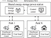Figure 1 Multi-park shared energy storage architecture.

After the distributed PV clusters are equipped with a shared ESS, the distributed PV can operate close to the maximum power point, while the ESS adjusts the power at the grid-connected connection points of the distributed PV clusters based on the system frequency deviation. The control center configures the corresponding energy storage capacity and arranges the charging and discharging power according to the electricity consumption behaviors of all parks and the needs of cluster users within a cycle. Park users are preferentially supplied with electricity by the distributed PV clusters, and the surplus electricity is sold to the shared energy storage power station, thereby improving the consumption level of distributed PV in the park. During the peak power generation period of the distributed PV clusters, park users purchase electricity from the shared energy storage power station to meet their own load demands, and the energy storage power station discharges to assist other PV clusters in making up for the power shortage in tracking the output plan. The shared energy storage power station mainly realizes profits through the price difference in purchasing and selling electricity at different times and charging service fees to the parks.

2.2.1 Objective function

The optimal configuration of energy storage should take into account two factors: firstly, the benefits of energy storage configuration for PV consumption in the distribution network should be considered [31]; on the other hand, the economic cost of energy storage configuration should also be considered [32]. Obviously, the higher the capacity of energy storage configuration, the better the effect of PV consumption, but the economic cost is also higher. Balancing the relationship between the consumption benefits and economic costs is one of the main issues discussed in this paper.

(1) The benefits of PV consumption

The benefits of PV consumption were set as objective 1, shown below:$$\max Z_1=\frac{\sum _{g\in {\mathrm{\Omega }}^P,t\in {\mathrm{\Omega }}^T,\omega \in {\mathrm{\Omega }}^S}\mathrm{}{P}_{p,t,s}^{\mathrm{PV}}}{P_p^{\mathrm{Max}}{\beta }_{t,s}},$$(8)where g, t, and ω are the indices of PV equipment, time periods, and scenarios, respectively; Ω ^P , Ω ^T , and Ω ^S are the collection of all PV devices, all time periods, and all scenes, respectively; $P_{p,t,s}^{\mathrm{PV}}$ is the actual power generated by PV, measured in MW; $P_p^{\mathrm{Max}}$ is the maximum output power of PV, measured in MW; β_t,s indicates the power output coefficient of PV, and is related to the sunshine intensity.

(2) The economic costs

The economic costs due to energy storage configuration were set as objective 2. To facilitate the economic assessment of shared ESS, the following assumptions are posited: (1) the investment cost of shared ESS exhibits a linear relationship with both unit power cost and unit energy cost; (2) the operational cost of energy storage is solely dependent on the unit power operational cost; and (3) the market electricity price remains constant, thereby maintaining a consistent charge/discharge price for energy storage. The specific mathematical model is detailed below:$$\min Z_2=\sum _{i={\mathrm{\Omega }}^{\mathrm{ESS}},\omega \in {\mathrm{\Omega }}^S}\mathrm{}{\chi }_{\omega }\left[\begin{array}{l}{C}^{E,\mathrm{ESS}}{x}_i^{\mathrm{ESS}}{E}^{\mathrm{ESS}}+C^{P,\mathrm{ESS}}{x}_i^{\mathrm{ESS}}{\bar{P}}^{\mathrm{ESS}}+C_{\omega }^{\mathrm{op}}{x}_i^{\mathrm{ESS}}{E}^{\mathrm{ESS}}+\\ \sum _{t\in {\mathrm{\Omega }}^T}\mathrm{}\left(C_{t,\omega }^{\mathrm{buy}}{P}_{i,t,\omega }^{S,C}-C_{t,\omega }^{\mathrm{DC}}{P}_{i,t,\omega }^{S,\mathrm{DC}}-C_{t,\omega }^{\mathrm{serve}}\right)\Delta t\\ \end{array}\right],$$(9)where $x_i^{\mathrm{ESS}}$ is the amount of energy storage configured in node i; E ^ESS is the capacity of unit energy storage; C ^E,ESS is the battery cost of energy storage; ${\bar{P}}^{\mathrm{ESS}}$ _{is the rated charge/discharge power of the unit energy storage device;} C ^P,ESS is the cost of the energy conversion system serving the energy storage and discharge; $C_{\omega }^{\mathrm{op}}$ is the maintenance cost per unit of energy storage for the scenario ω. $C_{t,\omega }^{\mathrm{buy}}$ and $C_{t,\omega }^{\mathrm{DC}}$ represent the unit prices for purchasing and selling electricity from shared energy storage, respectively, during time period t under scenario ω. $C_{t,\omega }^{\mathrm{serve}}$ signifies the service fee charged to users by the shared energy storage operator during time period t under scenario ω. $P_{i,t,\omega }^{S,\mathrm{DC}}$ and $P_{i,t,\omega }^{S,C}$ represent the discharging and charging power of the shared energy storage at node SS during time period t under scenario ω, respectively. The probability of scenario ω is represented by χ_ω, and Ω^ESS denotes the set of all candidate nodes for configuring energy storage.

The multi-objective optimization model includes multiple scenarios and multiple time periods, integrating the economics and energy efficiency of the ESS. The overall objective is to find an optimal balance between enhancing the benefits of PV consumption and controlling economic costs.

2.2.2 Constraints

(1) Coupling nodal power constraints

Constraints (10) and (11) limit active and reactive power transmission, respectively, at the grid coupling nodes. Constraints (12) and (13) are in the form of active and reactive power constraints at the coupling nodes [33, 34].$${\underset{ - }{P}}^{\mathrm{GSP}}\le P_{t,\omega }^{\mathrm{GSP}}\le {\overline{P}}^{\mathrm{GSP}}\hspace{1em}\forall t\in {\mathrm{\Omega }}^T,\hspace{1em}\forall \omega \in {\mathrm{\Omega }}^S$$(10) $${\underset{ - }{Q}}^{\mathrm{GSP}}\le Q_{t,\omega }^{\mathrm{GSP}}\le {\overline{Q}}^{\mathrm{GSP}}\hspace{1em}\forall t\in {\mathrm{\Omega }}^T,\hspace{1em}\forall \omega \in {\mathrm{\Omega }}^S$$(11) $$P_{t,\omega }^{\mathrm{GSP}}-\sum _{j\in {\mathrm{\Omega }}_a\left(i\right)}\mathrm{}{P}_{\mathrm{ij},t,\omega }^{\mathrm{line}}+P_{i,t,\omega }^{\mathrm{PV}}=P_{i,t,\omega }^D\hspace{1em}\forall t\in {\mathrm{\Omega }}^T,\hspace{1em}\forall \omega \in {\mathrm{\Omega }}^S$$(12) $$Q_{t,\omega }^{\mathrm{GSP}}-\sum _{j\in {\mathrm{\Omega }}_a\left(i\right)}\mathrm{}{Q}_{\mathrm{ij},t,\omega }^{\mathrm{line}}+Q_{i,t,\omega }^{\mathrm{PV}}=Q_{i,t,\omega }^D\hspace{1em}\forall t\in {\mathrm{\Omega }}^T,\hspace{1em}\forall \omega \in {\mathrm{\Omega }}^S$$(13)

where, $P^{\mathrm{GSP}}$ and ${\overline{P}}^{\mathrm{GSP}}$ are the minimum active power and maximum active power that can be transmitted by the coupling node, respectively; $Q^{\mathrm{GSP}}$ and ${\overline{Q}}^{\mathrm{GSP}}$ are the minimum reactive power and maximum reactive power that can be transmitted by the coupling node, respectively. P ^GSP and Q ^GSP are the active power and reactive power that can be transmitted by the coupling node, respectively. ${\mathrm{\Omega }}_a\left(i\right)$ is the set of the end node of the line with node as the first node; $P_{\mathrm{ij}}^{\mathrm{line}}$ and $Q_{\mathrm{ij}}^{\mathrm{line}}$ are the active power and reactive power on line ij, respectively; $P_i^D$and $Q_i^D$ are the active load and reactive load on node i, respectively. $P_i^{\mathrm{PV}}$ and $Q_i^{\mathrm{PV}}$ are the active power and reactive power injected by PV on node i, respectively.

(2) Power flow constraints

Constraints (14) and (15) represent the active and reactive power balance at the nodes. Constraints (16) represent the voltage landings on the line. Constraints (17) and (18) are the power constraints on the line, respectively.$$\begin{array}{l}\sum _{k\in {\mathrm{\Omega }}_f\left(i\right)}\mathrm{}\left[P_{\mathrm{ki},t,\omega }^{\mathrm{line}}-R_{\mathrm{ki}}{\left(I_{\mathrm{ki},t,\omega }^{\mathrm{line}}\right)}^2\right]-\sum _{j\in {\mathrm{\Omega }}_a\left(i\right)}\mathrm{}{P}_{\mathrm{ij},t,\omega }^{\mathrm{line}}+P_{i,t,\omega }^{\mathrm{PV}}+{\eta }_{\mathrm{DC}}{P}_{i,t,\omega }^{S,\mathrm{DC}}-P_{i,t,\omega }^{S,C}=P_{i,t,\omega }^D\\ \forall i\in {\mathrm{\Omega }}^B,\forall t\in {\mathrm{\Omega }}^T,\forall \omega \in {\mathrm{\Omega }}^S,\\ \end{array}$$(14) $$\sum _{k\in {\mathrm{\Omega }}_f\left(i\right)}\mathrm{}\left[Q_{\mathrm{ki},t,\omega }^{\mathrm{line}}-X_{\mathrm{ki}}{\left(I_{\mathrm{ki},t,\omega }^{\mathrm{line}}\right)}^2\right]-\sum _{j\in {\mathrm{\Omega }}_a\left(i\right)}\mathrm{}{Q}_{\mathrm{ij},t,\omega }^{\mathrm{line}}+Q_{i,t,\omega }^{\mathrm{PV}}=Q_{i,t,\omega }^D\hspace{1em}\forall i\in {\mathrm{\Omega }}^B,\hspace{1em}\forall t\in {\mathrm{\Omega }}^T,\hspace{1em}\forall \omega \in {\mathrm{\Omega }}^S,$$(15) $$\begin{array}{l}{\left(V_{i,t,\omega }\right)}^2-{\left(V_{j,t,\omega }\right)}^2=2\left(R_{\mathrm{ij}}{P}_{\mathrm{ij},t,\omega }^{\mathrm{line}}+X_{\mathrm{ij}}{Q}_{\mathrm{ij},t,\omega }^{\mathrm{line}}\right)-{\left(I_{\mathrm{ij},t,\omega }^{\mathrm{line}}\right)}^2\left[{\left(R_{\mathrm{ij}}\right)}^2+{\left(X_{\mathrm{ij}}\right)}^2\right]\\ \forall \mathrm{ij}\in {\mathrm{\Omega }}^{\mathrm{Line}},\hspace{1em}\forall t\in {\mathrm{\Omega }}^T,\hspace{1em}\forall \omega \in {\mathrm{\Omega }}^S,\\ \end{array}$$(16) $${\left(S_{\mathrm{ij},t,\omega }^{\mathrm{line}}\right)}^2={\left(P_{\mathrm{ij},t,\omega }^{\mathrm{line}}\right)}^2+{\left(Q_{\mathrm{ij},t,\omega }^{\mathrm{line}}\right)}^2\hspace{1em}\forall \mathrm{ij}\in {\mathrm{\Omega }}^{\mathrm{Line}},\hspace{1em}\forall t\in {\mathrm{\Omega }}^T,\hspace{1em}\forall \omega \in {\mathrm{\Omega }}^S,$$(17) $${\left(V_{i,t,\omega }\right)}^2{\left(I_{\mathrm{ij},t,\omega }^{\mathrm{line}}\right)}^2={\left(S_{\mathrm{ij},t,\omega }^{\mathrm{line}}\right)}^2\hspace{1em}\forall \mathrm{ij}\in {\mathrm{\Omega }}^{\mathrm{Line}},\hspace{1em}\forall t\in {\mathrm{\Omega }}^T,\hspace{1em}\forall \omega \in {\mathrm{\Omega }}^S,$$(18)

where, Ω^B is the set of nodes; Ω^Line is the collection of lines in the distribution network; R_ki, $R_{\mathrm{ij}}$, $X_{\mathrm{ki}}$, and $X_{\mathrm{ij}}$ are the resistance and reactance of the line ki and ij, respectively; ${\mathrm{\Omega }}_f\left(i\right)$ is the set of the first node of the line with node i as the end node; ${\mathrm{\Omega }}_a\left(i\right)$ is the set of the end node of the line with node as the first node; $I_{\mathrm{ki}}^{\mathrm{line}}$ and $I_{\mathrm{ij}}^{\mathrm{line}}$ are the currents flowing through the ki and ij lines, respectively; $P_{\mathrm{ij}}^{\mathrm{line}}$, $Q_{\mathrm{ij}}^{\mathrm{line}}$, and $S_{\mathrm{ij}}^{\mathrm{line}}$ are the active power, reactive power, and apparent power flowing on line ij, respectively; $P_{\mathrm{ki}}^{\mathrm{line}}$ and $Q_{\mathrm{ki}}^{\mathrm{line}}$ are the active power and reactive power on line ki, respectively; ${\eta }_{\mathrm{DC}}$ is the discharge efficiency of ESS; $P_i^{S,\mathrm{DC}}$ and $P_i^{S,C}$ are the discharge power and charging power of the ESS, respectively; V_i is the voltage of node i.

(3) PV power constraints

The inverter with the PV is able to realize the control of the power generated by the PV and to control the phase difference of the voltage and current to realize the control of the PV power factor, which enables the PV to work under the power factor of over- or under-lagging and is able to continuously control the power generated by itself. Constraints (19)–(21) limit the range of discarded power and operation of PV.$$P_{g,t,\omega }^{\mathrm{PV}}f\left(\underline{\theta }\right)\le Q_{g,t,\omega }^{\mathrm{PV}}\le P_{g,t,\omega }^{\mathrm{PV}}f\left(\bar{\theta }\right)\hspace{1em}\forall g\in {\mathrm{\Omega }}^G,\hspace{1em}\forall t\in {\mathrm{\Omega }}^T,\hspace{1em}\forall \omega \in {\mathrm{\Omega }}^S,$$(19) $$P_{g,t,\omega }^{\mathrm{PV}}=P_g^{\mathrm{Cap}}{\beta }_t-P_{g,t,\omega }^{\mathrm{Curt}}\hspace{1em}\forall g\in {\mathrm{\Omega }}^G,\hspace{1em}\forall t\in {\mathrm{\Omega }}^T,\hspace{1em}\forall \omega \in {\mathrm{\Omega }}^S,$$(20) $$0\le P_{g,t,\omega }^{\mathrm{Curt}}\le P_g^{\mathrm{Cap}}{\beta }_{t,\omega }\hspace{1em}\forall g\in {\mathrm{\Omega }}^G,\hspace{1em}\forall t\in {\mathrm{\Omega }}^T,\hspace{1em}\forall \omega \in {\mathrm{\Omega }}^S,$$(21)

where, $f\left(\underline{\theta }\right)$ and $f\left(\bar{\theta }\right)$ are the maximum and minimum power factor of the GTH PV, respectively; $P_{g,t,\omega }^{\mathrm{Curt}}$ is the abandoned light power of the PV;$P_g^{\mathrm{Cap}}$ is the rated power of PV, ${\beta }_t$ is the ratio of real output and rated power of PV, which varies along with the illumination.

(5) Voltage safety constraints

The safety constraint is characterized by equation (22). For the safety of the distribution network, the individual node voltages should be kept in a reasonable range.$${\underset{ – }{V}}_i\le V_{i,t,\omega }\le {\overline{V}}_i\hspace{1em}\forall i\in {\mathrm{\Omega }}^B,\hspace{1em}\forall t\in {\mathrm{\Omega }}^T,\hspace{1em}\forall \omega \in {\mathrm{\Omega }}^S,$$(22)

where, ${\underset{ - }{V}}_i$ and ${\overline{V}}_i$ are the minimum and maximum voltage levels of the i node, respectively.

(6) Shared ESS constraints

Constraints (23) and (24) indicate that the charging and discharging power of the ESS at any time period should not exceed its power limit. Constraints (25)–(27) indicate that the ESS cannot operate in the charging and discharging states simultaneously. Constraints (28)–(30) limit the state of charge of ESS.$$0\le P_{i,t,\omega }^{S,\mathrm{DC}}\le x_i^{\mathrm{ESS}}{\overline{P}}^{\mathrm{DC}}\hspace{1em}\forall i\in {\mathrm{\Omega }}^{\mathrm{ESS}},\hspace{1em}\forall t\in {\mathrm{\Omega }}^T,\hspace{1em}\forall \omega \in {\mathrm{\Omega }}^S,$$(23) $$0\le {\eta }_C{P}_{i,t,\omega }^{S,C}\le x_i^{\mathrm{ESS}}{\overline{P}}^C\hspace{1em}\forall i\in {\mathrm{\Omega }}^{\mathrm{ESS}},\hspace{1em}\forall t\in {\mathrm{\Omega }}^T,\hspace{1em}\forall \omega \in {\mathrm{\Omega }}^S,$$(24) $${\mu }_{i,t,\omega }^{\mathrm{DC}}+{\mu }_{i,t,\omega }^C\le 1\hspace{1em}\forall i\in {\mathrm{\Omega }}^{\mathrm{ESS}},\hspace{1em}\forall t\in {\mathrm{\Omega }}^T,\hspace{1em}\forall \omega \in {\mathrm{\Omega }}^{S,}$$(25) $$P_{i,t,\omega }^{S,\mathrm{DC}}\le M^{\mathrm{DC}}{\mu }_{i,t,\omega }^{\mathrm{DC}}\hspace{1em}\forall i\in {\mathrm{\Omega }}^{\mathrm{ESS}},\hspace{1em}\forall t\in {\mathrm{\Omega }}^T,\hspace{1em}\forall \omega \in {\mathrm{\Omega }}^S,$$(26) $$P_{i,t,\omega }^{S,C}\le M^C{\mu }_{i,t,\omega }^C\hspace{1em}\forall i\in {\mathrm{\Omega }}^{\mathrm{ESS}},\hspace{1em}\forall t\in {\mathrm{\Omega }}^T,\hspace{1em}\forall \omega \in {\mathrm{\Omega }}^S,$$(27) $$x_i^{\mathrm{ESS}}{\underline{S}}^{\mathrm{ESS}}\le S_{i,t,\omega }^{\mathrm{ESS}}\le x_i^{\mathrm{ESS}}{\overline{S}}^{\mathrm{ESS}}\hspace{1em}\forall i\in {\mathrm{\Omega }}^{\mathrm{ESS}},\hspace{1em}\forall t\in {\mathrm{\Omega }}^T,\hspace{1em}\forall \omega \in {\mathrm{\Omega }}^S,$$(28) $$S_{i,0,\omega }^{\mathrm{ESS}}=S_{i,N_T,\omega }^{\mathrm{ESS}}\hspace{1em}\forall \omega \in {\mathrm{\Omega }}^S,$$(29) $$S_{i,t,\omega }^{\mathrm{ESS}}=S_{i,t-1,\omega }^{\mathrm{ESS}}+{\eta }_C{P}_{i,t,\omega }^{S,C}-P_{i,t,\omega }^{S,\mathrm{DC}}\hspace{1em}\forall i\in {\mathrm{\Omega }}^{\mathrm{ESS}},\hspace{1em}\forall t\in {\mathrm{\Omega }}^T,\hspace{1em}\forall \omega \in {\mathrm{\Omega }}^S,$$(30)

where, ${\eta }_C$ is the charging efficiency of the ESS; ${\overline{P}}^{\mathrm{DC}}$ is the maximum charging power of the ESS; ${\mu }_{i,t,\omega }^{\mathrm{DC}}$ is the 0–1 variable that characterizes whether the ESS is in discharge state; ${\mu }_{i,t,\omega }^C$ is the 0–1 variable that characterizes whether the ESS is in the charging state; $S_{i,t,\omega }^{\mathrm{ESS}}$ is the state of charge of the energy storage device represents the stored energy; ${\overline{S}}^{\mathrm{ESS}}$ and ${\underline{S}}^{\mathrm{ESS}}$ are the maximum and minimum charge states of the energy storage device, respectively; MDC and MC are the numbers that are sufficiently large compared to $P_{i,t,\omega }^{S,\mathrm{DC}}$ and $P_{i,t,\omega }^{S,C}$, respectively.

(7) Network reconfiguration constraints

When a line blockage occurs in a major transmission line or a security overrun occurs, a reasonable reconfiguration of the network can improve the security level of the grid as well as the level of PV consumption. For a re-configurable grid, its state must satisfy two of the following three scenarios:

• Scenario A: Number of lines in service is 1 less than the number of nodes.

• Scenario B: There is no isolated grid.

• Scenario C: There is no ring network.

Constraints (31) give a more detailed mathematical description of Scenario A.$$\sum _{\mathrm{ij}={\mathrm{\Omega }}^{\mathrm{Line}}}\mathrm{}{a}_{\mathrm{ij},t}=N_{\mathrm{bus}}-1\hspace{1em}\forall t\in {\mathrm{\Omega }}^T,$$(31)

where $a_{\mathrm{ij}}$ represents the 0–1 variable of whether the line is in use. N_bus is the number of nodes in the distribution network.

The implementation of the distribution network reconfiguration model has transformed the power flow model significantly. For each node, utilizing the big-M method enabled the characterization of the operational line’s breaking state effectively as constraint (32). When the node is operational, the power flowing through the node is unrestricted; however, when the node is not in operation, the power on the node is zero. For each transmission line, the breakable line power flow calculation involves the following variations: constraint (33) illustrates the voltage relationship between the two ends of the interruptible line, with the voltage at both ends influenced by the basic circuit principle of the line when in operation. Constraints (34) and (35) describe the power relationship on the breakable line, while constraint (36) characterizes the current relationship on an interruptible line.$$-M^{\mathrm{im}}\cdot a_{\mathrm{ij},t}\le P_{\mathrm{ij},t}^{\mathrm{line}}\le M^{\mathrm{im}}\cdot a_{\mathrm{ij},t}\hspace{1em}\forall t,\hspace{1em}\forall \mathrm{ij}\in {\mathrm{\Omega }}^{\mathrm{Line}},$$(32) $$\begin{array}{l}\{\begin{array}{l}{\left(V_{i,t,\omega }\right)}^2-{\left(V_{j,t,\omega }\right)}^2\le M^V(1-a_{\mathrm{ij},t})+2(R_{\mathrm{ij}}{P}_{\mathrm{ij},t,\omega }^{\mathrm{line}}+X_{\mathrm{ij}}{Q}_{\mathrm{ij},t,\omega }^{\mathrm{line}})-{\left(I_{\mathrm{ij},t,\omega }^{\mathrm{line}}\right)}^2[{\left(R_{\mathrm{ij}}\right)}^2+{\left(X_{\mathrm{ij}}\right)}^2]\\ {\left(V_{i,t,\omega }\right)}^2-{\left(V_{j,t,\omega }\right)}^2\ge -M^V(1-a_{\mathrm{ij},t})+2(R_{\mathrm{ij}}{P}_{\mathrm{ij},t,\omega }^{\mathrm{line}}+X_{\mathrm{ij}}{Q}_{\mathrm{ij},t,\omega }^{\mathrm{line}})-{\left(I_{\mathrm{ij},t,\omega }^{\mathrm{line}}\right)}^2[{\left(R_{\mathrm{ij}}\right)}^2+{\left(X_{\mathrm{ij}}\right)}^2]\\ \end{array}\\ \forall \omega ,\hspace{1em}\forall t,\hspace{1em}\forall \mathrm{ij}\in {\mathrm{\Omega }}^{\mathrm{Line}},\\ \end{array}$$(33) $$-{\bar{P}}_{\mathrm{ij}}^{\mathrm{line}}\cdot a_{\mathrm{ij},t}\le P_{\mathrm{ij},t,\omega }^{\mathrm{line}}\le {\bar{P}}_{\mathrm{ij}}^{\mathrm{line}}\cdot a_{\mathrm{ij},t}\hspace{1em}\forall \omega ,\hspace{1em}\forall t,\hspace{1em}\forall \mathrm{ij}\in {\mathrm{\Omega }}^{\mathrm{Line}},$$(34) $$-{\bar{Q}}_{\mathrm{ij}}^{\mathrm{line}}\cdot a_{\mathrm{ij},t}\le Q_{\mathrm{ij},t,\omega }^{\mathrm{line}}\le {\bar{Q}}_{\mathrm{ij}}^{\mathrm{line}}\cdot a_{\mathrm{ij},t}\hspace{1em}\forall \omega ,\hspace{1em}\forall t,\hspace{1em}\forall \mathrm{ij}\in {\mathrm{\Omega }}^{\mathrm{Line}},$$(35) $$0\le {\left(I_{\mathrm{ij},t,\omega }^{\mathrm{line}}\right)}^2\le {\left({\bar{I}}_{\mathrm{ij}}^{\mathrm{line}}\right)}^2\cdot a_{\mathrm{ij},t}\hspace{1em}\forall \omega ,\hspace{1em}\forall t,\hspace{1em}\forall \mathrm{ij}\in {\mathrm{\Omega }}^{\mathrm{Line}},$$(36)

where, $M^{\mathrm{im}}$ and $M^V$ are relatively large constants; ${\bar{P}}_{\mathrm{ij}}^{\mathrm{line}}$ and ${\bar{Q}}_{\mathrm{ij}}^{\mathrm{line}}$ represent the maximum allowable active power and reactive power on line ij; ${\bar{I}}_{\mathrm{ij}}^{\mathrm{line}}$ represents the maximum allowable current flowing on line ij.

3 Optimization algorithm

The paper suggests utilizing the neural network algorithm to address the multi-objective problem by optimizing the Pareto optimal frontier. By integrating chaotic local search and quasi-adversarial learning techniques with the original neural network algorithm, a novel approach named the quasi-adversarial chaotic neural network algorithm is introduced to enhance the model’s effectiveness.

3.1 Basic neural network algorithm

3.1.1 Initialization

In the search space, the initial population X of pattern solutions is created randomly as follows:$$X=\left[\begin{array}{c}\begin{array}{ccc}{x}_1^1& x_2^1& \begin{array}{cc}\dots & x_N^1\end{array}\end{array}\\ \begin{array}{ccc}{x}_1^2& x_2^2& \begin{array}{cc}\dots & x_N^2\end{array}\end{array}\\ \begin{array}{c}\begin{array}{ccc}⋮& ⋮& \begin{array}{cc}⋮& ⋮\end{array}\end{array}\\ \begin{array}{ccc}{x}_1^{N_P}& x_2^{N_P}& \begin{array}{cc}\dots & x_N^{N_P}\end{array}\end{array}\end{array}\end{array}\right],$$(37)

where N_P is the population size; and N is the number of decision variables. After the initial population X is initialized, the objective function of the pattern solution is defined, and the best pattern solution with the best objective function value is the objective solution.

3.1.2 Weighted matrix of pareto optimality

The Pareto optimal frontier does not require the specification of weights for various objective functions; instead, it presents an array of outcomes resulting from assigning different weights within the weight matrix. In order to generate new candidate solutions, each pattern solution is assigned a corresponding weight vector with the following initial weights:$$W^t=\left[W_1,W_2,\dots ,W_{N_P}\right]=\left[\begin{array}{c}\begin{array}{ccc}{w}_1^1& w_2^1& \begin{array}{cc}\dots & w_N^1\end{array}\end{array}\\ \begin{array}{ccc}{w}_1^2& w_2^2& \begin{array}{cc}\dots & w_N^2\end{array}\end{array}\\ \begin{array}{c}\begin{array}{ccc}⋮& ⋮& \begin{array}{cc}⋮& ⋮\end{array}\end{array}\\ \begin{array}{ccc}{w}_1^{N_P}& w_2^{N_P}& \begin{array}{cc}\dots & w_N^{N_P}\end{array}\end{array}\end{array}\end{array}\right],$$(38)

where, W_t is a square matrix at the tth iteration that generates uniform random numbers from 0 to 1 over iterations.

In order to control the generation of new pattern solutions and shift bias, the sum of the weights of the pattern solutions is subject to the following constraints:$$\sum _{j=1}^{N_P}{w}_{\mathrm{ij}}^t=1\hspace{1em}i,j=\mathrm{1,2}, \dots ,N_P,$$(39)

where,$$w_{\mathrm{ij}}\in U\left[\mathrm{0,1}\right],\hspace{1em}i,j=\mathrm{1,2}, \dots ,N_P,$$(40)

The constraints in the above equation allow the pattern solution of the NNA to be generated with a slight deviation (from 0 to 1). After creating the initial weights, the weights corresponding to the target solution X_Target are selected from the weight matrix in equation (38) and are called target weights W_Target. Generate a new schema solution in the t+1st iteration and update the schema solution.$$X_{i,\mathrm{new}}^{t+1}=\sum _{\mathrm{j}=1}^{N_P}{w}_{\mathrm{ij}}^t\times X_i^t, \hspace{1em}j=\mathrm{1,2},\dots ,N_P,$$(41) $$X_i^{t+1}=X_i^t+X_{i,\mathrm{New}}^{t+1}, i=\mathrm{1,2},\dots ,N_P,$$(42) $$W_i^{t+1}=W_i^t+2\times \mathrm{rand}\left(\mathrm{0,1}\right)\times \left[W_{\mathrm{Target}}^t-W_i^t\right],\hspace{1em}i=\mathrm{1,2},\dots ,N_P.$$(43)

3.1.3 Bias term

A bias operator is used to adjust the probabilities of the pattern solutions created in the new population and in the updated weight matrix in order to update the search space. The bias operator serves to prevent the algorithm from converging prematurely, especially at the initial iteration.

In order to create a higher quality solution to the target solution, the update function transfers the new mode solution from the current location to a new location in the search space that is closer to the target solution. Therefore, the update function is defined as follows:$$X_{i,\mathrm{Updated}}^{t+1}=X_i^{t+1}+2\times \mathrm{rand}\left(\mathrm{0,1}\right)\times \left[X_{\mathrm{Target}}^t-X_i^{t+1}\right],\hspace{1em}i=\mathrm{1,2},\dots ,N_P,$$(44)

In the first iteration, the bias operator has more chances to create new pattern solutions to explore unknown pattern solutions. However, as the number of iterations increases, the bias operator has fewer chances and the transfer function operator has more chances to explore towards the target solution.

3.2 Opposition-based learning

The theory of Opposition-Based Learning (OBL) was first proposed by Tizhoosh [35]. The OBL strategy considers both the existing guesses and the opposite guesses to better approximate the existing candidate solutions. At the same time, quasi-opposite learning is more high-speed and efficient in obtaining the global optimal solution [36].

Based on the solution of the population model X_ij, the opposite of X_ij is $O{X}_{\mathrm{ij}}$ as follows:$$O{X}_{\mathrm{ij}}=L{B}_j+U{B}_j-X_{\mathrm{ij}}$$(45)

where, X_ij is the jth dimensional value of the current solution; $L{B}_j$ and $U{B}_j$ are the upper and lower bounds of the jth dimension.

The quasi-alignment site of $O{X}_{\mathrm{ij}}$ is $\mathrm{QO}{X}_{\mathrm{ij}}$ as follows:$$\mathrm{QO}{X}_{\mathrm{ij}}=\mathrm{rand}\left(\frac{L{B}_i+U{B}_i}{2},O{X}_{\mathrm{ij}}\right).$$(46)

In this paper, the QOBL algorithm encompasses two primary phases: population initialization and jump generation. Initially, during the population initialization phase, a quasi-oppositional population is generated alongside a randomly initialized population. The optimal solution for the initial population is then determined by evaluating both the randomly generated population and its quasi-oppositional counterpart. Subsequently, the jump generation phase facilitates the algorithm’s search process by potentially directing it towards quasi-positional solutions characterized by superior fitness function values. The jump rate, denoted as J_r, is employed to govern the decision between transitioning to the quasi-positional solution or retaining the current solution.

3.3 Chaotic local search

The inherent non-linearity and aperiodic nature of chaotic systems introduce a degree of randomness and exploratory behavior within the search space. This characteristic helps to circumvent the limitations of fixed patterns and periodic behaviors, thereby mitigating the risk of converging on local optima. In the QOCNNA method, the integration of CLS serves to prevent entrapment in local optima, enhance search diversity, improve search efficiency, and bolster global optimization capabilities, ultimately facilitating the discovery of the global optimum.

The initial chaotic values are defined as follows:$$Z_0=\mathrm{rand}\left(\mathrm{0,1}\right).$$(47)

The subsequent values of this chaotic sequence using the logistic map are shown in the following:$$Z_{k+1}=\mu \times Z_k\times \left(1-Z_k\right),$$(48)

where $Z_k\in \left(\mathrm{0,1}\right),\hspace{1em}\forall k\in \left\{\mathrm{0,1},2,...\right\}$ and $\mu \in \left(\mathrm{0,4}\right]$.

The CLS strategy speeds up the search process by exploring the neighborhood of the current target solution. As a result, the new candidate solutions are as follows [37]:$$X_{\mathrm{NewTarget},\mathrm{k}}=X_{\mathrm{Target},k}+\left(Z_k-0.5\right)\times \left(X_{i,k}-X_{j,k}\right)$$(49)

where X_Target,k and X_NewTarget,k are the current target solution and the new target solution created at the kth CLS iteration, respectively; X_i,k and X_j,k are two solutions randomly selected from the current population, respectively. Z_k is the chaos variable at the k iteration. If the value of the X_NewTarget,k fitness function is better than X_Target,k, it will be replaced in the population, and the CLS strategy will be executed until the CLS limit value (K) is satisfied.

3.4 Quasi-oppositional chaotic neural network algorithm

Initially, the QOCNNA algorithm generates a randomly initialized pattern solution X. Subsequently, QOBL is employed to construct a quasi-opposite population QOX for the initial population. The QOCNNA then combines X and QOX, selecting the top N_r solutions from the combined set {X, QOX} to constitute the initial population. The search process, analogous to NNA, is then executed to generate a new pattern solution population and update the weight matrix. Based on the jump rate J_r, QOBL facilitates the transition of QOCNNA towards superior quasi-opposite solutions of the current pattern solution. Finally, CLS is implemented to refine the objective solutions. The optimization process iterates until the stopping criteria are satisfied. T_max is the number of iterations. K is the limit value of iterations in CLS; The pseudocode for QOCNNA is presented in Table 1.

4 Solution processes

Each model solution of the initial population in QOCNNA represents the solution vector of the distributed PV network reconfiguration problem, which includes the switches turned on, the locations and sizes of the distributed patrons, and the i solution vector is represented as follows:$$X_i=\left[S_1,\dots ,S_{N_{\mathrm{SW}}},L_1,\dots ,L_{N_{\mathrm{PV}}},P_1,\dots ,P_{N_{\mathrm{PV}}}\right],$$(50)

where, S is opened switches; L is the location of DGs; P is the size of DGs; N_SW is the number of opened switches.

QOCNNA is randomly initialized as follows:$$S_i=\mathrm{round}\left[S_{i,\min }+\mathrm{rand}\left(\mathrm{0,1}\right)\times \left(S_{i,\max }-S_{i,\min }\right)\right],\hspace{1em}i=1,\dots ,N_{\mathrm{SW}},$$(51) $$L_j=\mathrm{round}\left[L_{j,\min }+\mathrm{rand}\left(\mathrm{0,1}\right)\times \left(L_{j,\max }-L_{j,\min }\right)\right],\hspace{1em}i=1,\dots ,N_{\mathrm{PV}},$$(52) $$P_j=\mathrm{round}\left[P_{j,\min }+\mathrm{rand}\left(\mathrm{0,1}\right)\times \left(P_{j,\max }-P_{j,\min }\right)\right],\hspace{1em}i=1,\dots ,N_{\mathrm{PV}},$$(53)

where, $S_{i,\min }$ is equal to 1; $S_{i,\max }$ is the length of the ith fundamental loop vectors. The principle of basic loop vectors can be found in the literature [38]. $L_{j,\min }$ is equal to 2 and indicates that DGs may be integrated to all buses except the slack bus. The specific flow chart is shown in Figure 2.

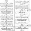Figure 2 The solution flow chart of QOCNNA.

5 Case study

5.1 Case settings

A modified IEEE 33-bus system, shown in Figure 3, is used for simulation verification. Employing the clustering methodology delineated in Section 2.1, the study area is partitioned into five distributed PV clusters as depicted in Figure 3. Shared ESS installation nodes are established between the campuses. The typical daily solar irradiance profiles and load profiles are illustrated in Figure 4. The solar irradiance profile represents the ratio of actual PV cluster output to the total installed PV capacity within the cluster, while the load profile indicates the ratio of actual load to the maximum load. The fundamental data for the shared ESS is presented in Table 2. The maximum number of daily line disconnections is set to four. The equivalent node of each distributed PV cluster is 1.5 MW of PV installed, and the investment economy is taken as the optimization objective, with the maximum discard rate set to 10%, which is simulated and verified.

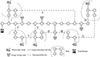Figure 3 33-bus study system.

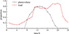Figure 4 Load and reference PV output curve.

To validate the efficacy of the proposed clustering method, a comparative analysis of power flow in the distribution network was conducted before and after PV equivalent modeling. The average relative errors of active power and node voltage at each time step are illustrated in Figure 5. Regarding the relative error of node voltage, all values are below 0.1%, with a daily average voltage error of 0.067%. As for the active power deviation, it remains below 0.1% during the 0-7 h period, with a daily average error of 0.49%, and a maximum value of 1.16% at 13 h. Consequently, the clustering equivalent effect of the method proposed in this paper demonstrates satisfactory accuracy.

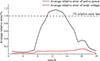Figure 5 Average relative error of active power and node voltage in different periods.

5.2 Analysis of ESS configuration results

In order to satisfy the goal of less than 10% abandonment rate, the minimum ESS investment cost is $3.4165×10⁶, and the results of ESS configuration are shown in Table 3.

According to Table 3, different nodes have different number of shared ESS units, with a minimum of 27 ESS devices installed at node 4 and a maximum of 49 ESS devices installed at node 13. This phenomenon is related to the network structure, which can be combined with the network structure diagram to show that the 4 node is the closest to the substation, while the 13 node is the furthest away from the substation. Since node 4 are electrically closer to the substation, when there is insufficient power in the system, it can directly transmit power from the substation to satisfy the power demand of the system; on the other hand, since the node 13 are electrically farther away from the substation, when there is insufficient power in the system, transmitting a large amount of power from the substation may result in voltage overruns that does not meet the safety requirements. Therefore, the further the electrical distance from the substation, the more ESS capacity is required to achieve local balancing of electrical energy and to reduce the operational stress of the ESS.

5.3 Analysis of network reconfiguration results

For the switches, they are numbered asⅠ-Ⅸ and their reconfiguration results are shown in Table 4.

As shown in Table 4, the network topology exhibits relative stability before the 8:00 and after 22:00. Conversely, the network topology undergoes frequent changes between 8:00 and 22:00. Furthermore, in conjunction with Figure 4, the output of the PV cluster gradually increases from the 8:00, peaking at the 13:00. The cluster output diminishes to zero after the 20:00, while the load remains at its peak between the 11:00 and 21:00. Consequently, a significant amount of PV power is injected back into the grid during the 8:00 to 22:00 due to the spatiotemporal mismatch between PV output and load demand. Network reconfiguration can mitigate issues such as line overload and voltage violations, thereby promoting the consumption of PV output. Conversely, the absence of PV output at night, coupled with a relatively stable load and the smoothing effect of ESS on load fluctuations, results in a more balanced line power distribution, significantly reducing the necessity for network topology adjustments. It is important to note that the solar irradiance and load curves in Figure 4 represent ratios relative to their maximum values, not actual values. Moreover, at 17:00, the maximum available PV power and system load are 3.75 MW and 2.1 MW, respectively, indicating that PV generation exceeds the load. At 18:00, the maximum available PV power and system load are 2.1 MW and 3.3435 MW, respectively, indicating that PV generation is less than the load. Therefore, topological changes are correlated with the matching degree between PV output and load.

The ESS at node 7 is in closer contact with the PV device at node 27. It can be seen that compared with node 4 and node 7, the ESS at node 13 and node 30 serve more parks, so the energy storage configuration results shown in Table 3, the energy storage installation at node 13 and node 30 is significantly higher than that at node 4 and node 7. This phenomenon also proves the effectiveness of the ESS configuration model proposed in this paper.

The integration of high-penetration distributed PV generation introduces challenges such as increased network losses, reverse power flow, and voltage violations. This section presents an analysis comparing network losses and nodal voltage variations before and after distribution network reconfiguration. The system’s network losses and nodal voltage profiles before and after reconfiguration are illustrated in Figures 6 and 7, respectively. Prior to reconfiguration, the total network loss was 0.739 MWh, which was reduced to 0.542 MWh post-reconfiguration, representing a 26.7% reduction. This indicates that the optimized reconfiguration strategy effectively mitigates system losses. Furthermore, the voltage at node 15 is closer to 1.0 p.u. after reconfiguration, demonstrating that network reconfiguration can alleviate voltage fluctuations caused by PV output and load variations, thereby contributing to improved voltage stability.

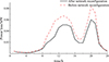Figure 6 Comparison of system losses before and after reconfiguration in different periods.

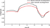Figure 7 Voltage comparison of node 15 before and after reconstruction in different periods.

5.4 Analysis of PV curtailment results.

In order to analyze the timing control state of each park PV cluster, the multi-time period simulation operation model is solved under the reference PV curve. The abandonment rate r can be calculated as follows:$$r=\frac{P_{g,t,\omega }^{\mathrm{Curt}}}{P_g^{\mathrm{Cap}}{\beta }_t}\times 100\%.$$(54)

Figure 8 shows the abandonment rate of each park PV cluster over 24 time periods, from which it can be seen that each node PV cluster has different degrees of abandonment from 8:00 to 16:00, especially at 9:00, when the abandonment rate reaches the maximum. Although the sunlight intensity reaches the maximum at 13:00, but 13:00 is also in the peak load time, obviously the abandoned light rate is not only related to the maximum power generation of PV cluster devices, but also related to the system load, and at 9:00, the light intensity to have been relatively high, while the system load is still in the growth stage. Therefore, at 9:00, the curtailment rate reaches the maximum.

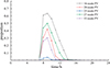Figure 8 The curtailment rate of each PV in each period.

On the other hand, it can be seen from Figure 8 that the 16-node PV cluster has the highest abandonment rate overall, followed by the 27-node, 20-node and 33-node, while the 25-node has the lowest abandonment rate, and in order to facilitate the explanation of this phenomenon, Figure 9. 6 demonstrates the load level of the parks in each of the 24 time periods. Comparing Figure 8 and Figure 9, it can be found that parks with higher loads have lower abandonment rates for their own PVs, especially the park where node 25 is located, whose overall load level is significantly higher than that of the other parks, and it can also be seen in Figure 8 that there is almost no abandonment of PVs cluster at node 25. This indicates that the parks with larger loads are able to better consume local PV power during the hours of stronger light, while the parks with smaller loads have to perform a large amount of discarding during the hours of stronger light due to network security constraints. This phenomenon further validates the effectiveness of the method proposed in this paper.

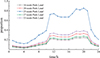Figure 9 The load of each park in each period.

5.5 Analysis of operation strategies of shared ESSs

The output of the four shared energy storage power stations in the multi-park during the operation period is shown in Figure 10, and their expenditure and income during a dispatch period are shown in Figure 11. Combined with Figures 10 and 11, it can be seen that at the peak of PV power generation, the park sells electricity to shared energy storage to absorb the excess power generation of the PV cluster, and purchases electricity from shared energy storage to meet its own needs when there is no sunshine or insufficient sunshine, and the load is strong. Among them, the shared energy storage on node 4 mainly meets the PV cluster consumption of nodes 20 and 25, as shown in Figure 10a. The shared energy storage on node 7 mainly meets the consumption of the PV cluster on node 27, as shown in Figure 10b. The shared energy storage on node 13 mainly meets the PV cluster consumption of node 16 and node 20, as shown in Figure 10c. The shared energy storage on node 30 mainly meets the PV cluster consumption of node 27 and node 33, as shown in Figure 10d.

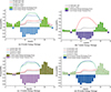Figure 10 The operating power of the shared energy storage station.

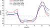Figure 11 The benefits of shared energy storage power stations.

5.6 Comparison with and without ESSs

To ascertain the influence of ESS on the absorption of PV clusters, an additional experiment was established, specifically excluding ESS configuration. Figures 8 and 12 present the curtailment outcomes with and without ESS, respectively. A comparative analysis of these results reveals that the implementation of ESS markedly diminishes the PV curtailment ratio. The primary timeframe for analyzing and contrasting the curtailment rates spans from 8:00 to 18:00, corresponding to periods of elevated solar irradiance and substantial PV output. In scenarios without ESS, the PV curtailment ratio escalates due to increased PV output, resulting in an inability to accommodate system load and subsequent network congestion. Post-18:00, PV power generation diminishes, and the generated power is directly consumed by the end-users. Furthermore, in conjunction with the ESS charging and discharging behavior depicted in Figure 1, the energy storage devices are observed to be charging between 8:00 and 18:00. After 18:00, the ESSs device initiate a significant discharge to satisfy the system’s load requirements. These observations suggest that, within systems characterized by high solar irradiance, the integration of energy storage facilitates the storage of electrical energy during periods of high solar intensity and its subsequent release during periods of low solar intensity, thereby enhancing the consumption of PV clusters.

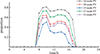Figure 12 curtailment rate in each period (without energy storage).

5.7 Analysis on pareto optimality

The Pareto front of the multi-objective model proposed in this paper is illustrated in Figure 13. A linear correlation is observed between investment cost and curtailment rate. The impact of shared energy storage systems on PV cluster integration is primarily reflected in the capacity and charge/discharge power of the storage. Based on the preceding analysis, the capacity of the energy storage system is the most significant factor influencing PV cluster integration. Even with an investment of $3.4165×10⁶, the simulated operation indicates that each energy storage device still reached its maximum state of charge. When energy storage is integrated into the system, the additional storage can accommodate surplus PV generation, thereby reducing curtailment. Consequently, a linear relationship exists between the curtailment rate and the investment cost. Furthermore, the Pareto curve is not entirely smooth, as shown in the figure, which is determined by the location of the shared energy storage devices. As indicated in the previous analysis, the radiation range of shared energy storage devices at each node varies, resulting in different benefits for the overall system’s PV integration when new storage is added at different nodes.

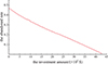Figure 13 The Pareto Frontier.

5.8 Analysis of 69-bus system

The modified IEEE 69-bus system is used to verify that when w₁ and w₂ take 0.5 respectively, the division of the distributed PV cluster is shown in Figure 14. Each PV is installed with a 500 kW PV. Taking the investment economy as the optimization objective, and setting the maximum light rejection rate of 10%, the simulation verification is carried out.

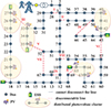Figure 14 IEEE69 node example system.

As shown in Table 5, the energy storage allocation predominantly favors the terminal nodes. This outcome stems from the higher concentration of distributed PV installations at these nodes, necessitating increased energy storage capacity for effective PV resource absorption. Due to the considerable distance from the substation, transmitting substantial electrical power may result in voltage violations, thereby compromising secure operational standards. Consequently, the terminal nodes could be primarily supplied by ESS to mitigate line power transmission and minimize losses.

For the 10 switches in Figure 14, numbered I-X, the branch numbers put into use in each period are shown in Table 6.

The topological structure’s variation pattern in Table 6 mirrors that observed in IEEE 33 bus system. Given the unchanged profiles of PV output and load demand, the network topology remains relatively stable before 8:00 and after 22:00. Conversely, the network topology undergoes more frequent changes between 8:00 and 22:00. These topological alterations are strongly correlated with the matching degree between PV output and load demand.

6 Conclusion

This paper introduces a multi-objective optimization configuration method for shared energy storage, considering network reconfiguration and equivalent clustering of PV. An improved QOCNNA is employed to solve the proposed model. Finally, the proposed method is applied to test systems of varying scales. The conclusions drawn are as follows:

1. When the output of PV generation does not match the load demand, it is necessary to fully utilize network reconfiguration and the charge/discharge capabilities of energy storage to absorb PV generation, ensuring the secure operation of the power grid.

2. The integration of shared energy storage devices is an efficient solution for the absorption of PV clusters. By storing electrical energy during periods of high solar irradiance and grid absorption difficulties, and releasing energy during periods of low generation, the method promotes PV absorption and mitigates fluctuations in the power system .

3. The Pareto optimal solution set for shared energy storage planning, obtained from the model in terms of PV absorption and the economic viability of energy storage investment, can provide practical guidance for energy storage planning in real-world engineering applications.

Funding

The authors declare that financial support was received for the research, authorship, and/or publication of this article. This paper is supported by the project of Economic Research Institute of State Grid Hebei Electric Power Co., Ltd., grant number is KJ2023-020.

References

All Tables

All Figures

	Figure 1 Multi-park shared energy storage architecture.
In the text

	Figure 2 The solution flow chart of QOCNNA.
In the text

	Figure 3 33-bus study system.
In the text

	Figure 4 Load and reference PV output curve.
In the text

	Figure 5 Average relative error of active power and node voltage in different periods.
In the text

	Figure 6 Comparison of system losses before and after reconfiguration in different periods.
In the text

	Figure 7 Voltage comparison of node 15 before and after reconstruction in different periods.
In the text

	Figure 8 The curtailment rate of each PV in each period.
In the text

	Figure 9 The load of each park in each period.
In the text

	Figure 10 The operating power of the shared energy storage station.
In the text

	Figure 11 The benefits of shared energy storage power stations.
In the text

	Figure 12 curtailment rate in each period (without energy storage).
In the text

	Figure 13 The Pareto Frontier.
In the text

	Figure 14 IEEE69 node example system.
In the text

References

- Huang N, Zhao X, Guo Y, Cai G, Wang R (2023) Distribution network expansion planning considering a distributed hydrogen-thermal storage system based on photovoltaic development of the Whole County of China, Energy 278, 127761. https://doi.org/10.1016/j.energy.2023.127761. [Google Scholar]
- Mohamad F, Teh J, Lai C-M (2021) Optimum allocation of battery energy storage systems for power grid enhanced with solar energy, Energy 223, 120105. https://doi.org/10.1016/j.energy.2021.120105. [Google Scholar]
- Lim KZ, Lim KH, Wee XB, Li Y, Wang X (2020) Optimal allocation of energy storage and solar photovoltaic systems with residential demand scheduling, Applied Energy 269, 115116. https://doi.org/10.1016/j.apenergy.2020.115116. [Google Scholar]
- Ren Y, Jin K, Gong C, Hu J, Liu D, Jing X, Zhang K (2023) Modelling and capacity allocation optimization of a combined pumped storage/wind/photovoltaic/hydrogen production system based on the consumption of surplus wind and photovoltaics and reduction of hydrogen production cost, Energy Convers. Manag. 296, 117662. https://doi.org/10.1016/j.enconman.2023.117662. [Google Scholar]
- Yao J, Xiao C, Hao J, Yang X (2024) Research on power consumption data prediction of distributed photovoltaic power station, HighTech Innov. J. 5(4), 937–948. https://doi.org/10.28991/HIJ-2024-05-04-05. [Google Scholar]
- Bozsik N, Szeberényi A, Bozsik N (2024) Impact of Climate Change on the Performance of Household-Scale Photovoltaic Systems, HighTech Innov. J., 5(1), 1–15. https://doi.org/10.28991/HIJ-2024-05-01-01. [Google Scholar]
- Chen Y, Liu F, Wei W, Mei S (2021) Energy sharing at demand side: concept, mechanism and prospect, Dianli Xitong Zidonghua/Autom. Electric Power Syst 45(2), 1–11. https://doi.org/10.7500/AEPS20200506004. [Google Scholar]
- Han O, Ding T, Zhang X, Mu C, He X, Zhang H, Jia W, Ma Z (2023) A shared energy storage business model for data center clusters considering renewable energy uncertainties, Renew. Energy 202, 1273–1290. https://doi.org/10.1016/j.renene.2022.12.013. [Google Scholar]
- Xie Y, Luo Y, Li Z, Xu Z, Li L, Yang K (2022) Optimal allocation of shared energy storage considering the economic consumption of microgrid new energy, Gaodianya Jishu/High Volt. Eng. 48(11), 4403–4412. https://doi.org/10.13336/j.1003-6520.hve.20220403. [Google Scholar]
- Ma M, Huang H, Song X, Peña-Mora F, Zhang Z, Chen J (2022) Optimal sizing and operations of shared energy storage systems in distribution networks: A bi-level programming approach, Appl. Energy 307, 118170. https://doi.org/10.1016/j.apenergy.2021.118170. [Google Scholar]
- Wang J, Zhao L, Lu H, Wei C (2024) Multi-objective stochastic-robust based selection-allocation-operation cooperative optimization of rural integrated energy systems considering supply-demand multiple uncertainties, Renew. Energy 233, 121159. https://doi.org/10.1016/j.renene.2024.121159. [Google Scholar]
- Ren F, Lin X, Ma X, Wei Z, Wang R, Zhai X (2023)A two-stage planning method for design and dispatch of distributed energy networks considering multiple energy trading, Sustain. Cities Soc. 96, 104666. https://doi.org/10.1016/j.scs.2023.104666. [Google Scholar]
- Xiong YF, Chen LJ, Zhen TW, Si Y, Mei SW (2021)Optimal configuration of hydrogen energy storage in low-carbon park integrated energy system considering electricity-heat-gas coupling characteristics, Electric Power Autom. Equip. 41(9), 31–38. [Google Scholar]
- Chen C, Liu C, Ma L, Chen T, Wei Y, Qiu W, Lin Z, Li Z (2023) Cooperative-game-based joint planning and cost allocation for multiple park-level integrated energy systems with shared energy storage, J. Energy Storage 73, 108861. https://doi.org/10.1016/j.est.2023.108861. [Google Scholar]
- Xu W, Yang Y, Zhang L, Xia Y, LI K (2025) Bi-level planning strategy for distribution network based on source-load temporal characteristics, Proc. CSU-EPSA 37(1), 17–25. https://doi.org/10.19635/j.cnki.csu-epsa.001444. [Google Scholar]
- Adnan, Nisar N, Shah RH, Zada FM, Khan B, Aziz S, Rehman NU, Soonmin H, Ahmad N, Khan M, Hanzala (2024) Novel Ni/ZnO nanocomposites for the effective photocatalytic degradation of malachite green dye, Civil Eng. J.-Tehran 10, 8, 2601–2614. https://doi.org/10.28991/CEJ-2024-010-08-011. [Google Scholar]
- Chen L, Sun Y, Wu Z, Ye L, Shi Y, Li Z (2023) Distributed PV cluster partitioning strategy based on GAN data synthesis federation clustering, in: 2023 8th International Conference on Power and Renewable Energy, ICPRE 2023, pp. 1730–1735. https://doi.org/10.1109/ICPRE59655.2023.10353797. [Google Scholar]
- Ding M, Zhang Y, Bi R, Hu D, Gao P (2021) Coordinated grid-power source expansion planning for distribution network considering cluster partition, Proc. CSEE 33, 1, 136–143. https://doi.org/10.19635/j.cnki.csu-epsa.000487. [Google Scholar]
- Cotilla-Sanchez E, Hines PDH, Barrows C, Blumsack S, Patel M (2013) Multi-attribute partitioning of power networks based on electrical distance, IEEE Trans. Power Syst. 28, 4, 4979–4987. https://doi.org/10.1109/TPWRS.2013.2263886. [Google Scholar]
- Liang J, Zhou J, Yuan X, Huang W, Gong X, Zhang G (2024) An active distribution network voltage optimization method based on source-network-load-storage coordination and interaction, Energies 17, 18, 4645. https://doi.org/10.3390/en17184645. [Google Scholar]
- Sheng H, Zhu Q, Tao J, Zhang H, Peng F (2024) Distribution network reconfiguration and photovoltaic optimal allocation considering harmonic interaction between photovoltaic and distribution network, J. Electric. Eng. Technol. 19, 1, 17–30. https://doi.org/10.1007/s42835-023-01506-y. [Google Scholar]
- Hachemi AT, Sadaoui F, Saim A, Ebeed M, Arif S (2024) Dynamic operation of distribution grids with the integration of photovoltaic systems and distribution static compensators considering network reconfiguration, Energy Rep. 12, 1623–1637. https://doi.org/10.1016/j.egyr.2024.07.050. [Google Scholar]
- Li H, Lekic A, Li S, Jiang D, Guo Q, Zhou L (2023) Distribution network reconfiguration considering the impacts of local renewable generation and external power grid. IEEE Trans. Indus. Appl. 59, 6, 7771–7788. https://doi.org/10.1109/TIA.2023.3307070. [Google Scholar]
- Liao CF, Tan Y, Li Y, Cao YJ (2022) Optimal operation for hybrid AC and DC systems considering branch switching and VSC control. IEEE Syst. J. 16, 4, 6708–6716. https://doi.org/10.1109/JSYST.2022.3151342. [Google Scholar]
- Li H, Ji CX, Xiang DW, Cheng RJJ (2023) A switching oscillation event-triggered switch fault detection method for SiC DC-DC converter, IEEE Trans. Indus. Electron. 70, 7, 7323–7333. https://doi.org/10.1109/TIE.2022.3220823. [Google Scholar]
- Yu H, Li H, Wang H, Li S (2024) Optimal configuration of fault location measurement points in DC distribution networks based on improved particle Swarm Optimization Algorithm, Energy Eng. J. Assoc. Energy Eng. 121, 6, 1535–1555. https://doi.org/10.32604/ee.2024.046936. [Google Scholar]
- Phommixay S, Doumbia ML, St-Pierre DL (2020) Review on the cost optimization of microgrids via particle swarm optimization, Int. J. Energy Environ. Eng. 11, 1, 73–89. https://doi.org/10.1007/s40095-019-00328-7. [Google Scholar]
- Rajalakshmi K, Priyan SV, Inbakumar JP, Kumar C (2024) Enhancing efficiency in electrical distribution systems: A novel approach via modified genetic optimization algorithm for loss reduction in optimal network distribution, J. Inte. Fuzzy Syst. 46, 2, 3577–3591. https://doi.org/10.3233/JIFS-231234. [Google Scholar]
- Li Q, Shao YQ, Liu HL, Shao XD (2020) Multi-objective optimization of activation time and discharge time of thermal battery using a genetic algorithm approach, Energies 13, 24, 6477. https://doi.org/10.3390/en13246477. [Google Scholar]
- Brusco MJ, Steinley D, Watts AL (2023) On maximization of the modularity index in network psychometrics, Behav. Res. Methods 55, 7, 3549–3565. https://doi.org/10.3758/s13428-022-01975-5. [Google Scholar]
- Ma L, Li W, Pei W, Xiao H, Ju L, Gu J (2024) Hybrid energy storage configuration optimization in distribution network with high-proportion PV considering demand response, Gaodianya Jishu/High Volt. Eng. 50, 4, 1416–1425. https://doi.org/10.13336/j.1003-6520.hve.20230593. [Google Scholar]
- Yu QH, Tian L, Li XD, Tan X (2022) Compressed air energy storage capacity configuration and economic evaluation considering the uncertainty of wind energy, Energies 15, 134637. https://doi.org/10.3390/en15134637. [Google Scholar]
- Grisales-Noreña LF, Morales-Duran JC, Velez-Garcia S, Montoya OD, Gil-González W (2023) Power flow methods used in AC distribution networks: An analysis of convergence and processing times in radial and meshed grid configurations, Results Eng. 17, 100915. https://doi.org/10.1016/j.rineng.2023.100915. [Google Scholar]
- Taheri B, Molzahn DK (2024) AC power flow informed parameter learning for DC power flow network equivalents, in: 2024 IEEE Texas Power and Energy Conference, TPEC 2024. https://doi.org/10.1109/TPEC60005.2024.10472173. [Google Scholar]
- Tizhoosh HR (2005) Opposition-based learning: A new scheme for machine intelligence, in: Proceedings - International Conference on Computational Intelligence for Modelling, Control and Automation, CIMCA 2005 and International Conference on Intelligent Agents, Web Technologies and Internet, 1, pp. 695–701. [Google Scholar]
- He G, Lu X (2023) Quasi opposite-based learning and double evolutionary QPSO with its application in optimization problems, Eng. Appl. Artif. Inte. 126, 106861. https://doi.org/10.1016/j.engappai.2023.106861. [Google Scholar]
- Zhou X, Gui W, Heidari AA, Cai Z, Liang G, Chen H (2023) Random following ant colony optimization: Continuous and binary variants for global optimization and feature selection, Appl. Soft Comput. 144, 110513. https://doi.org/10.1016/j.asoc.2023.110513. [Google Scholar]
- Sedighizadeh M, Esmaili M, Esmaeili M (2014) Application of the hybrid big bang-big crunch algorithm to optimal reconfiguration and distributed generation power allocation in distribution systems. Energy 76, 920–930. https://doi.org/10.1016/j.energy.2014.09.021. [Google Scholar]