")
")
| Issue |
Sci. Tech. Energ. Transition
Volume 81, 2026
|
|
|---|---|---|
| Article Number | 2 | |
| Number of page(s) | 10 | |
| DOI | https://doi.org/10.2516/stet/2026002 | |
| Published online | 06 March 2026 | |
Regular Article
Impact of connected vehicles on the traffic efficiency and PM emissions of mixed traffic flows
Intelligent Social Computing Lab, College of Physics and Electronic Engineering, Sichuan Normal University, Chengdu 610101, PR China
* Corresponding author: This email address is being protected from spambots. You need JavaScript enabled to view it.
Received:
17
July
2024
Accepted:
27
January
2026
Abstract
With the rapid development of Connected Vehicles (CVs), it is inevitable that Human-driven Vehicles (HVs) and CVs run on the same road in the near future. Besides the traffic efficiency, the sustainable development in society has become more and more concerned with Particulate Matter (PM) emissions very recently. In this work, mixed traffic flows with both CVs and HVs on a two-lane expressway are proposed; the effects of CV penetration rate on the traffic flow, and the PM emission are the focus. The results of the numerical simulation show that the traffic flow is effectively improved as the proportion of CVs increases. However, there are two stages of PM emissions. When the density is lower, the greater the proportion of CVs, the lower the PM emissions. When the density is higher, the situation reverses. Furthermore, traffic flows in two lanes are not the same, and the symmetry is terribly broken when the penetration of CVs is high. In terms of the forward observable interval of CVs, it can limit PM emissions and increase traffic flow. Thus, a high traffic efficiency and a low PM emission require a high CV penetration but an appropriate observable interval.
Key words: Connected vehicles / Human-driven vehicles / Mixed traffic flows / Particulate Matter (PM) emissions
© The Author(s), published by EDP Sciences, 2026
 This is an Open Access article distributed under the terms of the Creative Commons Attribution License (https://creativecommons.org/licenses/by/4.0), which permits unrestricted use, distribution, and reproduction in any medium, provided the original work is properly cited.
1 Introduction
With the development of the urban economy, the number of vehicles has increased rapidly. Traffic congestion has become more and more serious and has also contributed to the emission of Particle Matter (PM) [1–5]. These sustainability problems pose a threat to the environment [6]. Road traffic is the main contributor to PM emissions in urban cities [7]. Therefore, there is a growing need to develop sustainable and environmentally friendly urban road transport systems. In urban transport systems, expressways are an important component of vehicle travel. However, traffic congestion occurs frequently on highways, causing wasted travel time, traffic accidents, and high PM emissions [8, 9]. Frequent traffic congestion on urban expressways poses significant challenges to traffic management and environmental protection.
However, benefiting from advances in vehicle networking communication technology, as a product combining the automobile industry and emerging technologies, Connected Vehicles (CVs) have developed rapidly worldwide [10, 11]. On the one hand, CVs are expected to improve the operational quality of traffic flow from the micro-vehicle level and alleviate the current traffic congestion problem through Vehicle-to-Vehicle (V2V) and Vehicle-to-Infrastructure (V2I) technologies [12–18]. On the other hand, the application of CVs can reduce transportation emissions [19]. Compared to Human-driven Vehicles (HVs), CVs can perceive the environment with more accuracy and perform coordinated control [20, 21]. As the market penetration rate of CVs is gradually increasing, the transition towards a fully autonomous road system would require a considerable amount of time. Within this transition period, we can see that HVs and CVs run on the same road [22]. Therefore, it is of great significance to study the mixed traffic flow composed of CVs and HVs. This is a prerequisite before formed pure CV on the road [23, 24]. As the two types of vehicles have different behavioural characteristics, when they interact with each other, the mixed traffic flows formed may present characteristics not seen in pure HV traffic flows [25, 26].
To mitigate the impact of CVs on the road as soon as possible, scholars have conducted many simulation analyses on the running characteristics of CVs under Vehicle-to-Vehicle (V2V) environment, including road capacity and pollutant emissions. A large number of existing studies have proposed different physics-based models to replicate the car-following and lane-changing behaviors of HVs and CVs in the mixed traffic flow [27–30]. Among many of the physics-based models, the Cellular Automata (CA) model is a very flexible and efficient in calculation. It can factually simulate complex traffic phenomena by simple rules and consider many complex factors [31–33]. Specifically, Chen et al. proposed a CA model to analyze the influence of the degree of foresight and the ratio of CVs on traffic capacity [34]. Hu et al. constructed a CA model in which CV forward movement rules were derived based on the dynamic headway, considering the vehicles’ driving performance [35]. Liu et al. introduced a probability parameter in the deceleration rule and analyzed collision risks in mixed traffic flows [36]. Jiang et al. focused on the safety distance for mixed traffic flow that contains HVs, CVs, and CV platoons and proposed a CA model that different kinds of cars have a different calculation method for safety distance [37]. Yang et al. proposed a two-lane CA model that captured the differences between HVs and CVs [38]. Hua et al. proposed a multi-lane CA model to analyze the influence of lane policies on mixed traffic flows with various traffic volumes and CV penetration rates [39]. Liu et al. proposed a CA model that considered the lane changing of vehicles. This model was applied to evaluate the impact of different lane-changing behavior on traffic flow in a three-lane expressway [40].
In addition, Many researchers have conducted research on transportation emissions of transportation systems [41–43] Stogios et al. explored the effects of Automated Vehicles (AVs) and Electric Vehicles (EVs) on transportation emissions based on microscopic traffic simulation and emissions models [44]. The result showed that different Automated Vehicle (AV) strategies have different effects on emissions. Moreover, the result means that a good AV strategy can reduce emissions; on the contrary, it may increase emissions. A dynamic distributed routing algorithm was proposed by Tu et al. to reduce greenhouse gases for Connected and Automated Vehicles (CAVs) [45]. The results indicated that with the increase of CAVs, the NOx emission decreases significantly. Xiao et al. investigated the emissions of a hybrid traffic flow consisting of electric vehicles and conventional fuel vehicles, and comparatively analyzed the effect of the mixed ratio on the overall emissions [46]. In light of these considerations, Coppola et al. (2022) proposed an eco-driving control architecture for platoons of heterogeneous, nonlinear connected autonomous electric vehicles under uncertain conditions. Their research demonstrates that by employing a combination of Model Predictive Control (MPC) and Deep Reinforcement Learning (DRL), it is possible to manage the unique characteristics of heterogeneous vehicles, improving energy efficiency and reducing emissions through Vehicle-to-Everything (V2X) communication [47]. Furthermore, Li et al. (2023) evaluated the benefits of CVs in mixed traffic flows, finding that increasing the proportion of CVs can significantly reduce fuel consumption and emissions, particularly during congested traffic conditions. Their findings highlight the importance of understanding and optimizing mixed traffic scenarios to maximize environmental benefits [48].
The above research shows that CA models can effectively simulate mixed traffic flows and be applied to study the PM emissions on the road. However, the existing research only considers the surrounding vehicle information, and does not consider the vehicle information over long distances. This makes the operating mechanism analysis of mixed traffic flows appear inaccurate. This article discusses traffic flow and PM emissions based on the mixed situation of CVs and HVs. The main contributions of this paper are summarized as follows.
-
Time Headway (TH) and Time to Collision (TC) of CVs are introduced in the car-following model of CVs. In the lane-changing behaviour of CVs, CVs consider lane-changing incentive criteria for the forward observable interval based on the Symmetric Two-lane Cellular Automata (STCA);
-
The influence of penetration rate of CVs on traffic flow is discussed from the aspects of the fundamental diagram and PM emission;
-
Analyzing the driving efficiency of different lanes with the same proportion of CVs and same forward observable interval;
-
In the case of the same proportion of CVs, the impact of traffic conditions and PM emissions on the lane under different forward observable intervals.
The result of this paper is structured as follows. Section 2 introduces different models that are used in CVs and HVs. In Section 3, the simulation results of mixed traffic flows are analyzed. Finally, the conclusion is given in Section 4, and future work directions are put forward.
2 Model
In this work, we study a two-lane traffic flow CA model with two types of vehicles and their PM emission, based on a Symmetric Two-lane Cellular Automata (STCA) model [31, 32], and the schematic diagram is shown in Figure 1. There are two parallel lanes in the model, and each lane is composed of L cells. Each cell has two states at any time. One is occupied because there is a vehicle, the other is vacant because there is no vehicle here. There are two types of vehicles, one is a Human-driven Vehicle (HV), and the other is Connected Vehicle (CV). Both types of vehicles obey two behaviors in sequence, the lane-changing behaviors and the car-following behaviors. But HVs and CVs follow different rules, and the following subsections show them in detail.
 |
Figure 1 Car-following scenarios in mixed traffic flow. |
2.1 Human-driven vehicle model
The car-following rule of HVs is based on the NaSch model [33] when the inner or external cause for random braking is considered. HVs run in a single parallel lane according to the following four rules,
• Acceleration: (1)
(1)
• Deceleration: (2)
(2)
• Randomization with probability p: (3)
(3)
• Movement of vehicles: (4)
(4)
where v n (t) and x n (t) denote the speed and position of the vehicle n at time step t respectively. d n = x n−1 − x n − l n−1 is the free space in front of the vehicle n and l n−1 is the length of the vehicle n − 1. p denotes the randomization probability and vmax is the maximum allowed speed.
The lane-changing rule of HVs follows the STCA model proposed by Rickert et al. [31],
• Incentive criteria: (5)
(5)
• The safety criteria: (6)where d
n,other is the free space in front of the vehicle n on the other lane. Where d
n,back is the free space behind the vehicle n on the other lane. dsafe is the safe space, and set the value of dsafe to vmax. As shown in Figure 1, the HV n will change its lane to the other one and wants to reach a higher speed when the lane-changing rule is met.
(6)where d
n,other is the free space in front of the vehicle n on the other lane. Where d
n,back is the free space behind the vehicle n on the other lane. dsafe is the safe space, and set the value of dsafe to vmax. As shown in Figure 1, the HV n will change its lane to the other one and wants to reach a higher speed when the lane-changing rule is met.
2.2 Connected vehicle model
CVs can get more information through the Internet, such as the velocities of vehicles ahead. Drivers can drive their vehicles more aggressively according to the threat assessment [49] after being informedabout their local environments. The threat assessment is measured by the Time Headway (TH) [50–52]. TH is the time for the following vehicle to reach the momentary position of its front vehicle, (7)
(7)
TH has not used the velocity information of the vehicle ahead. It just measures the remaining time as the safest strategy for drivers to stop their vehicles at the current speed. For the highest traffic efficiency of the following vehicles under a safe condition without breaking, the following CVs should be better at catching the speed of their front vehicles. As it is assumed in the NaSch model where vehicle can always slow down their speed to a safe one, CVs behave more aggressively in a safe manner to catch up to their front vehicles’ speed. Thus, the Time to Collision (TC) is introduced to measure the time needed for the focus vehicle to speed up to the front vehicle’s current speed with the maximum acceleration amax. It can be written as (8)
(8)
TC < 0 means the front vehicle with a slower speed than the focus one, and the focus vehicle should not be too aggressive. While TC > 0 means the front vehicle with a higher speed and the focus one can still boost its speed. When TC < TH, it means that the vehicle can catch up to the speed of the front vehicle at the maximum acceleration within a time not exceeding TH. In this case, the vehicle can safely boost its speed. Here, we set the maximum acceleration amax = 2, which permits the vehicle to speed up to a higher speed. When TC > TH, it means that even if the vehicle catches up to the speed of the preceding vehicle at maximum acceleration, it may cause a collision. Therefore, the vehicle should adjust acceleration more carefully (reduce or maintain the same, here choose to maintain the same) to ensure safety. Therefore, the following rule is modified as,
• Acceleration: (9)
(9)
• Deceleration: (10)
(10)
• Movement of vehicles: (11)
(11)
HVs tend to change their lanes once their front distances cannot allow them to accelerate. What they only know is that the front distance on the other lane is longer in current time. This means that HVs are short-sighted. However, CVs are not. They can not only obtain the current speed of their front vehicles, but also all the speeds and positions of vehicles in front of their L
s
distance both on their lanes and on the other lanes. They will use more information to decide whether to change their lanes. Considering that the average speed describes the traffic efficiency, CVs mainly compare the average speed in front L
s
distance of two lanes. In many cases, numbers of vehicles in L
s
distances on these two lanes are not exactly the same. mother(t) is the number of vehicles on the other lane in the interval L
s
and n(self)(t) is the number of vehicles on the current lane in the interval L
s
. Then, the average speeds on these two lanes are (12)
(12)
 (13)
(13)
If vother (t) > vself (t), the focus vehicle prefers moving onto the other lane. Otherwise, they prefer the current lane. In this article, the CV lane changing rule modified from STCA is
• Incentive criteria: (14)
(14)
• The safety criteria: (15)
(15)
2.3 Emission model
In this work, traffic PM emissions on expressways are also considered [53], where the emission model proposed by Panis et al. is involved with the velocity and the acceleration, and it is derived from the nonlinear multivariate regression of real urban driving conditions [54]. The calculation formula is as follows,![Mathematical equation: $$ \begin{array}{lll}{E}_n(t)& =& \mathrm{max}[{E}_0,{f}_1+{f}_2{v}_n(t)+{f}_3{v}_n^2(t)\\ & +& {f}_4{a}_n(t)+{f}_5{a}_n^2(t)+{f}_6{v}_n(t){a}_n(t)]\end{array}, $$](/articles/stet/full_html/2026/01/stet20240244/stet20240244-eq16.gif) (16)where E
n
(t) is the pollutant emission for the vehicle n in unit time. E0 is a lower limit of emission (g/s) specified for each vehicle and pollutant type, and f1 to f6 are emission parameters specific for each vehicle and pollutant type, determined by the regression analysis. All of the specified parameters value is given in Table 1.
(16)where E
n
(t) is the pollutant emission for the vehicle n in unit time. E0 is a lower limit of emission (g/s) specified for each vehicle and pollutant type, and f1 to f6 are emission parameters specific for each vehicle and pollutant type, determined by the regression analysis. All of the specified parameters value is given in Table 1.
3 Results and analyses
In the CA model, the road segment is subdivided into cells and time into time steps. At each time step, each cell has only two states, which are either occupied by a vehicle or are empty. Each cell corresponds to 7.5 m and the maximum velocity is vmax = 5 cells per simulation steps, which corresponds to 135 km/h in the real world. The simulation is carried out on two-lane road segments, in which each lane is composed of 1000 cells, under periodic boundary conditions, which reduces the boundary effect and mimics an infinitely large system. The number of vehicles on each lane is denoted as N, all HVs have the same randomization probability p = 0.25. The observation interval L
s
for connected vehicles is equal to 100 cells. The CV penetration rate r is defined as the percentage of the number of connected vehicle in all the vehicles. The CV penetration rate r = 0, 0.2, 0.4, 0.6, 0.8, 1. The average vehicle emissions and the average velocity are obtained in the process of simulations by averaging over 30 independent initial realizations up to 4000 iteration steps T for each run and by discarding the first 2000 iteration steps as a transient time t0. The average velocity  of traffic flow is defined as follows,
 (17)
(17)
The fundamental diagram of mixed traffic flows is obtained for different mixing ratio r by numerical simulations. The global density is (18)
(18)
The mixed flow is defined as follows. (19)
(19)
In order to determine overall vehicle PM emissions, the average vehicle PM emission is defined as follows. (20)where E
n(t) represents the pollutant emission of the vehicle n at time t.
(20)where E
n(t) represents the pollutant emission of the vehicle n at time t.
3.1 Simulation results of the mixed traffic flow
Figure 2 depicts the volume–density and velocity–density diagrams of mixed traffic flow. In Figure 2a, at the beginning, the impact of r on the traffic flow J is very small. This means there are few vehicles on the road and the interaction between vehicles is small; they can move at their preferred speeds without being influenced by other vehicles. The traffic flow increases along with the density, until it reaches the critical density point. After that, the traffic flow decreases when vehicles are not free to drive. Furthermore, a higher CV penetration rate r supports a higher traffic efficiency. That is, the higher the proportion of CVs, the more efficient the traffic flow. Figure 2b shows the result that the average velocity of vehicles at different traffic densities for the different penetration rates. At low density, there are only a few vehicles on the road, and vehicles are free to drive. While the density increases, vehicles should consider the state of their front vehicles and the penetration rate r affects the average speed. A higher penetration rate r allows a little bit higher average speed. Specifically, when r is set to 1, the road is fully occupied by CVs without random braking; vehicles can travel at maximum speed.
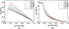 |
Figure 2 The fundamental diagram of the mixed traffic flow. (a) the diagram of volume–density, and (b) the diagram of velocity–density. |
Figure 3a shows the average emission of PM for mixed flows. In the case of low density, vehicles are free to drive. Because CVs are without randomization, the acceleration and deceleration behavior is less. As PM emissions equation (16) are mainly generated by the vehicle speed, the greater the penetration of CVs, the less PM emissions from the road. With the increase in density, the situation is gradually reversed, a higher penetration rate of CVs, the more PM emissions. This is because the more CVs there are, the more acceleration and deceleration behaviors there are, which alleviates the decrease in average velocity, but also causes an increase in PM emission. When the road is full of CVs, the PM emissions are close to twice as high the PM emissions without full CVs.
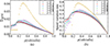 |
Figure 3 (a) PM emissions-Density diagram of mixed traffic flow. (b) Speed variation rate diagram of mixed traffic flow. |
In order to further study the PM characteristics of mixed traffic flows, the motion state of vehicles is divided into acceleration behavior (v n (t + 1) > v n (t)), deceleration behavior (v n (t + 1) < v n (t)) and uniform behavior (v n (t + 1) = v n (t)). Figure 3b shows the percentage of speed variation against the global density ρ. In a low-density environment, the higher penetration of CVs, the smaller the proportion of speed variation, indicating that most of the vehicles on the road are driving at a constant high speed, which can be seen in Figure 2b. When the roads are full of CVs, the speed variation proportion is 0, indicating that all vehicles on the road are driving at a constant speed at maximum speed. As the density increases, more CVs lead to a higher proportion of acceleration. As similar average speeds for different penetrations, there will also be a much higher proportion of speed variation. A high density needs that vehicles pay more attention to front vehicles. Therefore, vehicles with higher r will have a higher average speed. A higher average speed and more frequent speed variation will lead to a much higher average emissions as shown in Figure 3a.
3.2 Symmetry breaking in two lanes
In ordinary works for traffic flows on two lanes [31, 37], traffic flows on two lanes show little difference. However, the symmetry is broken for the mixed traffic flow. Figures 4a and 4b show the maximum difference between lane density and the maximum difference between lane average velocity with different CV penetrations, respectively. To be remembered, the penetration rate r = 0 means all vehicles are HVs and r = 1 is for all CVs. In these cases, the symmetry remains and the difference in lane density is caused by the fluctuation of the finite size. However, when 0 < r < 1 the traffic flow is with both HVs and CVs, the symmetry breaks, and it is obviously shown in Figure 4a with r = 0.6 and r = 0.8. A lower density ρ provide much larger spaces among vehicles and a much higher ρ will leads to much more traffic jams and even traffic blocks, which makes mechanisms of CVs and HVs have little effect. In the interval of the density ρ ∈ [0.2, 0.6] the lane density difference is visible in Figure 4a. This means the number of vehicles on one lane is much larger than that on the other lane. The maximum difference between lane average speeds on two lanes in Figure 4b is similar with that of the lane density difference. The maximum speed difference means that traffic flows on different lanes are quite different, which suggests the traffic flow on one lane is much more efficient than that on the other one.
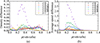 |
Figure 4 (a) Maximum lane density difference with different CV penetrations. (b) Maximum lane average speed difference with different CV penetration. |
The average velocity, the Speed variation rate, and the PM emission of each lane are shown in Figure 5 with the penetration rate of CVs r = 0.8. When the density is very low or high, the speeds, Speed variation rate, and PM emissions on two lanes are relatively close. At a density in [0.2, 0.5], the situation is not the same for the two lanes. Measures on one lane are larger than those on the other lane. It shows that symmetries on different measures are terribly broken, where the fluctuation does not diminish. It is quite intuitive that the asymmetry in this interval will be shown in each evolution of numerical simulations.
 |
Figure 5 The CV penetration rate of r = 0.8 on two lane. (a) Velocity-Density diagram, (b) Speed variation rate diagram, and (c) PM-emissions diagram. |
Figure 6 shows space-time diagrams of one evolution for mixed traffic flow on two lanes. The subplots in the same row are space-time diagrams on lane 1 and lane 2 respectively. The first row (a1) and (a2) is for the global density ρ = 0.16 with the CVs penetration r = 0.8 and the second row (b1) and (b2) is for ρ = 0.16 and r = 1. The last rows are for ρ = 0.3 fixed, r = 0.8 within (c1) and (c2) and r = 1 within (d1) and (d2) respectively. At a certain time step a red dot in each subplot shows a CV is at the position and a blue dot is for an HV. It shows clearly in Figures 6a1 and 6a2 that more HVs on the lane 1 than on the lane 2 with mixed vehicles. The traffic congestion is caused by HVs due to the randomization. However, the congestion spots are eased and even disappear due to CVs. The average velocity  on lane 1 is obversely smaller than
  on lane 2, which indicates that more HVs on a lane will lead to a slower average velocity on this lane due to the randomization of HVs. In contrast, when all vehicles are CVs, the traffic flow on two lanes is with the same velocity
  , which is the maximum velocity of vehicles, shown in Figures 6b1 and 6b2. The space-time diagram for this case shows almost a homogeneous distribution of dots on subplots. When the density is higher, e.g. ρ = 0.3, there are too many vehicles to support vehicles to run at their highest velocity. For the mixed traffic case with r = 0.8 in Figures 6c1 and 6c2, it is more obvious that more HVs are on the lane 1 with a slower average velocity
  and fewer HVs but most CVs are on lane 2 with a much higher average velocity
  , which is quite close to the average velocity of the case where vehicles are all CVs in Figures 6d1 and 6d2.
 |
Figure 6 Space-time diagrams of mixed traffic flow after the transient time. (a) with ρ = 0.16, r = 0.8, (b) with ρ = 0.16, r = 1, (c) with ρ = 0.3, r = 0.8, and (d) ρ = 0.3, r = 1. |
The asymmetry is not just about the average velocity but also the lane density. Remembering the average velocity of the whole vehicles r = 1 are quite close to the case r = 0.8 shown in Figure 2b and that the penetration r = 0.8 means that HVs are only a small proportion of vehicles and CVs are the most proportion, it is obviously that the lane density on lane 2 is much larger than the lane density on lane 1. Thus, the lane density symmetry is also hardly broken. While r = 1 without the disturbance of HVs, once the congestion is formed, it is maintained by the traffic of CVs.
3.3 Different forward observable interval
Effects of the forward observable interval L
s
on the PM emission  and the traffic flow J are with the penetration rate r = 0.6 shown in Figure 7. It shows that a Larger value of the observable interval helps the traffic flow pollutes less emissions, characterized by the maximum
  . The larger the observable distance in front of the vehicle, the greater the flow rate and the smaller the pollutant emissions. Too short a forward observable length does not benefit from less pollution. The insect shows that the critical density for
  reaching a maximum is increasing along with the increase of L
s
. Correspondingly, Figure 7b shows L
s
shows less effect on the traffic flow J but much higher than r = 0 in Figure 2a. Thus, a proper forward observable interval can help vehicles pollute less without affecting the traffic efficiency.
reaching a maximum is increasing along with the increase of L
s
. Correspondingly, Figure 7b shows L
s
shows less effect on the traffic flow J but much higher than r = 0 in Figure 2a. Thus, a proper forward observable interval can help vehicles pollute less without affecting the traffic efficiency.
 |
Figure 7 (a) Maximum PM emissions under different forward observableinterval and the inset is the diagram of PM–density under different forward observable interval. (b) Maximum traffic flow under different forward observable interval and the inset is diagram of volume–density under different forward observable interval. |
4 Conclusion
In this work, a mixed traffic flow with connected vehicles (CVs) and human-driven vehicles (HVs) is investigated by the numerical simulation of the cellular automata. The traffic efficiency and the PM emission are the focus of this work. CVs and HVs obey different lane-changing and car-following mechanisms. Besides, CVs can boost their speed faster than HVs due to the car-following mechanisms; CVs are without randomization. Thus, a higher penetration of CVs supports a higher traffic efficiency but more PM emissions. Furthermore, when CVs and HVs coexist on the road, CVs prefer avoiding the lane where more HVs are. Considering that the lane-changing mechanism of CVs needs the local lane efficiency, described by the average velocity of vehicles in the forward observable interval, it makes CVs play a long-sighted lane-changing rule. In contrast, HVs only considering the front vehicle is a short-sighted lane-changing rule. This makes the change lane behavior of CVs more efficient. When the density is a medium value, the traffic is get congestion. As all vehicles tend to change to a faster lane to reach a faster speed, it results in a faster lane with a higher lane density while the slower lane has a lower lane density. However, it is known to all that higher lane density will lead to a lower traffic efficiency, i.e., a slower average velocity. Therefore, the role of the two lanes exchanges. After many times of reorganizations, a dynamic tradeoff of the mixed traffic in the steady state is that most HVs are on a lane to reach a higher speed. Symmetries of lane velocities and lane densities are broken. This is the reason why a higher penetration makes the traffic reach a higher average velocity and flow. However, a higher speed and frequent speed up after lane changing make CVs contribute much more to the PM permission.
Expanding upon our preliminary work, future research can delve into a broader range of traffic scenarios, including autonomous vehicles with varying levels of driving capabilities and V2X communication technologies, as explored in [55]. This expansion would incorporate more environmental variables and vehicle behavior models, while also allowing for a nuanced analysis of emissions, as explored in [56]. Additionally, the optimization of driving strategies for autonomous vehicles, inspired by [57], could be central to reducing emissions while maintaining traffic efficiency. The long-term effects of differing autonomous vehicle penetration rates on traffic patterns, infrastructure adaptability, and communication reliability will also be subjects of further inquiry. These studies, collectively, will offer deep insights and recommendations critical to the evolution of intelligent transportation systems.
References
- Yang L., Chau K.W., Szeto W.Y., Cui X., Wang X. (2020) Accessibility to transit, by transit, and property prices: Spatially varying relationships, Transp. Res. Part D 85, 102387. [Google Scholar]
- Van Fan Y., Perry S., Klemeš J.J., Lee C.T. (2018) A review on air emissions assessment: Transportation, J. Clean. Prod. 194, 673–684. [Google Scholar]
- Lu Q.Y., Chai J., Wang S., Zhang Z.G., Sun X.C. (2020) Potential energy conservation and CO2 emissions reduction related to China’s road transportation, J. Clean. Prod. 245, 118892. [Google Scholar]
- Bao Z.K., Ou Y.F., Chen S.Z., Wang T. (2022) Land use impacts on traffic congestion patterns: A tale of a Northwestern Chinese City, Land 11, 12, 2295. [Google Scholar]
- Bao Z.K., Ng S.T., Yu G., Zhang X.L., Ou Y.F. (2023) The effect of the built environment on spatial-temporal pattern of traffic congestion in a satellite city in emerging economies, Dev. Built Environ. 14, 100173. [Google Scholar]
- Sohrabi S., Khreis H., Lord D. (2020) Impacts of autonomous vehicles on public health: A conceptual model and policy recommendations, Sustain. Cities Soc. 63, 102457. [Google Scholar]
- Zhang Z.Y., Song G.H., Zhai Z.Q., Li C.X., Wu Y.Z. (2019) How many trajectories are needed to develop facility-and speed-specific vehicle-specific power distributions for emission estimation? Case study in Beijing, Transp. Res. Rec. 2673, 11, 779–790. [Google Scholar]
- Xie R., Fang J.Y., Liu C.J. (2017) The effects of transportation infrastructure on urban carbon emissions, Appl. Energy 196, 199–207. [Google Scholar]
- Li X.P., Cui J.X., An S., Parsafard M.S. (2014) Stop-and-go traffic analysis: Theoretical properties, environmental impacts and oscillation mitigation, Transp. Res. Part B 70, 319–339. [Google Scholar]
- Montanaro U., Dixit S., Fallah S., Dianati M., Stevens A., Oxtoby D., Mouzakitis A. (2019) Towards connected autonomous driving: review of use-cases, Veh. Syst. Dyn. 57, 6, 779–814. [Google Scholar]
- Bansal P., Kockelman K.M.(2017) Forecasting Americans’ long-term adoption of connected and autonomous vehicle technologies, Transp. Res. Part A 95, 49–63. [Google Scholar]
- Sharma A., Zheng Z.D., Kim J., Bhaskar A., Haque M.M. (2021) Assessing traffic disturbance, efficiency, and safety of the mixed traffic flow of connected vehicles and traditional vehicles by considering human factors, Transp. Res. Part C 124, 102934. [Google Scholar]
- Carrone A.P., Rich J., Vandet C.A., An K. (2021) Autonomous vehicles in mixed motorway traffic: capacity utilisation, impact and policy implications, Transport. 48, 2907–2938. [Google Scholar]
- Yao Z.H., Hu R., Jiang Y.S., Xu T.R. (2020) Stability and safety evaluation of mixed traffic flow with connected automated vehicles on expressways, J. Safety Res. 75, 262–274. [Google Scholar]
- Yao Z.H., Gu Q.F., Jiang Y.S., Ran B. (2022) 549 Fundamental diagram and stability of mixed traffic flow 550 considering plato on size and intensity of connected auto-551 mated vehicles, Physica A 604, 127857. [Google Scholar]
- Yao Z.H., Wu Y.X., Jiang Y.S., Ran B. (2022) Modeling the fundamental diagram of mixed traffic flow with dedicated lanes for connected automated vehicles, IEEE Trans. Intell. Transp. Syst. 24, 6, 6517–6529. [Google Scholar]
- Zheng L., Zhu C., He Z.B., He T. (2021) Safety rule-based cellular automaton modeling and simulation under V2V environment, Transportmetrica A 17, 1, 81–106. [Google Scholar]
- Wang M., Hoogendoorn S.P., Daamen W., van Arem B., Shyrokau B., Happee R. (2018) Delay-compensating strategy to enhance string stability of adaptive cruise controlled vehicles, Transportmetrica B 6, 3, 211–229. [Google Scholar]
- Yao Z.H., Wang Y., Liu B., Zhao B., Jiang Y.S. (2021) Fuel consumption and transportation emissions evaluation of mixed traffic flow with connected automated vehicles and human-driven vehicles on expressway, Energy 230, 120766. [Google Scholar]
- Talebian A., Mishra S. (2018) Predicting the adoption of connected autonomous vehicles: A new approach based on the theory of diffusion of innovations, Transp. Res. Part C 95, 363–380. [Google Scholar]
- Jiang Y.S., Zhao B., Liu M., Yao Z.H. (2021) A two‐level model for traffic signal timing and trajectories planning of multiple CAVs in a random environment, J. Adv. Transp. 1, 1. [Google Scholar]
- Mahbub A.M.I., Malikopoulos A.A. (2021) Conditions to provable system-wide optimal coordination of connected and automated vehicles, Automatica 131, 109751. [Google Scholar]
- Yao Z.H., Xu T.R., Jiang Y.S., Hu R. (2021) Linear stability analysis of heterogeneous traffic flow considering degradations of connected automated vehicles and reaction time, Physica A 561, 125218. [Google Scholar]
- Yao Z.H., Jiang H.R., Jiang Y.S., Ran B. (2023) A two-stage optimization method for schedule and trajectory of CAVs at an isolated autonomous intersection, IEEE Trans. Intell. Transp. Syst. 24, 3, 3263–3281. [Google Scholar]
- Xiao L., Wang M., van Arem B. (2019) Traffic flow impacts of converting an HOV lane into a dedicated CACC lane on a freeway corridor, IIEEE Intell. Transp. Syst. Mag. 12, 1, 60–73. [Google Scholar]
- Liu H., Kan X.A., Shladover S.E., Lu X.Y., Ferlis R.E. (2018) Impact of cooperative adaptive cruise control on multilane freeway merge capacity, J. Intell. Transp. Syst. 22, 3, 263–275. [Google Scholar]
- Liu K.Y., Feng T.J. (2023) Heterogeneous traffic flow cellular automata model mixed with intelligent controlled vehicles, Physica A 632, 1, 129316. [Google Scholar]
- Jin S., Sun D.H., Zhao M., Li Y., Chen J. (2020) Modeling and stability analysis of mixed traffic with conventional and connected automated vehicles from cyber physical perspective, Physica A 551, 124217. [Google Scholar]
- Cao Z.P., Lu L.L., Chen C., Chen X.U. (2021) Modeling and simulating urban traffic flow mixed with regular and connected vehicles, IEEE Access 9, 10392–10399. [Google Scholar]
- Ozkan M.F., Ma Y. (2021) Modeling driver behavior in car-following interactions with automated and human-driven vehicles and energy efficiency evaluation, IEEE Access 9, 64696–64707. [Google Scholar]
- Rickert M., Nagel K., Schreckenberg M., Latour A. (1996) Two lane traffic simulations using cellular automata, Physica A 231, 4, 534–550. [Google Scholar]
- Chowdhury D., Wolf D.E., Schreckenberg M. (1997) Particle hopping models for two-lane traffic with two kinds of vehicles: Effects of lane-changing rules, Physica A 235, 3–4, 417–439. [Google Scholar]
- Nagel K., Schreckenberg M. (1992) A cellular automaton model for freeway traffic, J. Phys. I 2, 12, 2221–2229. [Google Scholar]
- Chen D.J., Ahn S.Y., Chitturi M., Noyce D.A. (2017) Towards vehicle automation: Roadway capacity formulation for traffic mixed with regular and automated vehicles, Transp. Res. Part B 100, 196–221. [Google Scholar]
- Hu X.H., Huang M.Y., Guo J.P. (2020) Feature analysis on mixed traffic flow of manually driven and autonomous vehicles based on cellular automata, Math. Probl. Eng. 1, 7210547. [Google Scholar]
- Liu Y., Lin X., He F., Li M. (2018) Cellular automata for modeling safety issues in mixed traffic of conventional and autonomous vehicles, in: Wang X.K., Zhang Y., Yang D.G., You Z. (eds), 18th COTA International Conference of Transportation Professionals, CICTP 2018, Reston, Beijing, China, pp. 56–65. [Google Scholar]
- Jiang Y.J., Wang S.C., Yao Z.H., Zhao B., Wang Y. (2021) A cellular automata model for mixed traffic flow considering the driving behavior of connected automated vehicle platoons, Physica A 582, 126262. [Google Scholar]
- Yang D., Qiu X.P., Ma L., Wu D.H., Zhu L.L., Liang H.B. (2017) Cellular automata–based modeling and simulation of a mixed traffic flow of manual and automated vehicles, Transp. Res. Rec. 2622, 1, 105–116. [Google Scholar]
- Hua X.D., Yu W.J., Wang W., Xie W.J. (2020) Influence of lane policies on freeway traffic mixed with manual and connected and autonomous vehicles, J. Adv. Transp. 1, 3968625. [Google Scholar]
- Liu Y.Z.X., Guo J.Q., Taplin J., Wang Y.B. (2017) Characteristic analysis of mixed traffic flow of regular and autonomous vehicles using cellular automata, J. Adv. Transp. 1, 8142074. [Google Scholar]
- Zhang X.Q., Li L., Zhang J. (2019) An optimal service model for rail freight transportation: Pricing, planning, and emission reducing, J. Clean. Prod. 218, 565–574. [Google Scholar]
- Xie R., Fang J.Y., Liu C.J. (2017) The effects of transportation infrastructure on urban carbon emissions, Appl. Energy 196, 199–207. [Google Scholar]
- Pan W., Xue Y., He H.D., Lu W.Z. (2018) Impacts of traffic congestion on fuel rate, dissipation and particle emission in a single lane based on Nasch Model, Physica A 503, 154–162. [Google Scholar]
- Stogios C., Kasraian D., Roorda M.J., Hatzopoulou M. (2019) Simulating impacts of automated driving behavior and traffic conditions on vehicle emissions, Transp. Res. Part D 76, 176–192. [Google Scholar]
- Tu R., Alfaseeh L., Djavadian S., Farooq B., Hatzopoulou M. (2019) Quantifying the impacts of dynamic control in connected and automated vehicles on greenhouse gas emissions and urban NO2 concentrations, Transp. Res. Part D 73, 142–151. [Google Scholar]
- Xiao H., Huang H.J., Tang T.Q. (2017) Analysis of energy consumption and emission of the heterogeneous traffic flow consisting of traditional vehicles and electric vehicles, Mod. Phys. Lett. B 31, 34, 1750324. [Google Scholar]
- Coppola A., Lui D.G., Petrillo A., Santini S. (2022) Eco-driving control architecture for platoons of uncertain heterogeneous nonlinear connected autonomous electric vehicles, IEEE Trans. Intell. Transp. Syst. 23, 12, 24220–24234. [Google Scholar]
- Li H.G., Li H.T., Hu Y., Xia T., Miao Q., Chu J. (2023) Evaluation of fuel consumption and emissions benefits of connected and automated vehicles in mixed traffic flow, Front. Energy Res. 11, 1207449. [Google Scholar]
- Johnsson C., Laureshyn A., De Ceunynck T.D. (2018) In search of surrogate safety indicators for vulnerable road users: a review of surrogate safety indicators, Transport Rev. 38, 6, 765–785. [Google Scholar]
- Siebert F.W., Oehl M., Pfister H.R. (2014) The influence of time headway on subjective driver states in adaptive cruise control, Transp. Res. Part F 25, 65–73. [Google Scholar]
- Arrouch I., Ahmad N.S., Goh P., Mohamad-Saleh J. (2022) Close proximity time-to-collision prediction for autonomous robot navigation: an exponential GPR approach, Alex. Eng. J. 61, 12, 11171–11183. [Google Scholar]
- Lu C.R., Dong J., Houchin A., Liu C.H. (2021) Incorporating the standstill distance and time headway distributions into freeway car-following models and an application to estimating freeway travel time reliability, J. Intell. Transp. Syst. 25, 1, 21–40. [Google Scholar]
- Wang X., Xue Y., Cen B.L., Zhang P. (2020) Study on pollutant emissions of mixed traffic flow in cellular automaton, Physica A 537, 122686. [Google Scholar]
- Panis L.I., Broekx S., Liu R.H. (2006) Modelling instantaneous traffic emission and the influence of traffic speed limits, Sci. Total Environ. 371, 1–3, 270–285. [Google Scholar]
- Pan Y., Wu Y., Xu L., Xia C., Olson D.L. (2024) The impacts of connected autonomous vehicles on mixed traffic flow: A comprehensive review. Physica A Stat. Mech. Appl. 635, 129454. [Google Scholar]
- Zhang T., Zhan J., Shi J., Xin J., Zheng N. (2023) Human-like decision- making of autonomous vehicles in dynamic traffic scenarios. IEEE CAA J. Autom. Sinica 10, 10, 1905–1917. [Google Scholar]
- Sognnaes I., Gambhir A., van de Ven D.J., Nikas A., Anger-Kraavi A., Bui H., Campagnolo L., Delpiazzo E., Doukas H., Giarola S., Grant S., Hawkes A., Köberle A.C., Kolpakov A., Mittal S., Moreno J., Perdana S., Rogelj J., Vielle M., Peters G.P. (2021). A multi-model analysis of long-term emissions and warming implications of current mitigation efforts. Nat. Clim. Chang. 11, 12, 1055–1062. [Google Scholar]
All Tables
All Figures
|
Figure 1 Car-following scenarios in mixed traffic flow. |
| In the text | |
|
Figure 2 The fundamental diagram of the mixed traffic flow. (a) the diagram of volume–density, and (b) the diagram of velocity–density. |
| In the text | |
|
Figure 3 (a) PM emissions-Density diagram of mixed traffic flow. (b) Speed variation rate diagram of mixed traffic flow. |
| In the text | |
|
Figure 4 (a) Maximum lane density difference with different CV penetrations. (b) Maximum lane average speed difference with different CV penetration. |
| In the text | |
|
Figure 5 The CV penetration rate of r = 0.8 on two lane. (a) Velocity-Density diagram, (b) Speed variation rate diagram, and (c) PM-emissions diagram. |
| In the text | |
|
Figure 6 Space-time diagrams of mixed traffic flow after the transient time. (a) with ρ = 0.16, r = 0.8, (b) with ρ = 0.16, r = 1, (c) with ρ = 0.3, r = 0.8, and (d) ρ = 0.3, r = 1. |
| In the text | |
|
Figure 7 (a) Maximum PM emissions under different forward observableinterval and the inset is the diagram of PM–density under different forward observable interval. (b) Maximum traffic flow under different forward observable interval and the inset is diagram of volume–density under different forward observable interval. |
| In the text | |
Current usage metrics show cumulative count of Article Views (full-text article views including HTML views, PDF and ePub downloads, according to the available data) and Abstracts Views on Vision4Press platform.
Data correspond to usage on the plateform after 2015. The current usage metrics is available 48-96 hours after online publication and is updated daily on week days.
Initial download of the metrics may take a while.