")
")
| Issue |
Sci. Tech. Energ. Transition
Volume 79, 2024
Power Components For Electric Vehicles
|
|
|---|---|---|
| Article Number | 5 | |
| Number of page(s) | 9 | |
| DOI | https://doi.org/10.2516/stet/2023039 | |
| Published online | 16 janvier 2024 | |
Regular Article
AC motor impedance predictive modeling methodology taking into account windings variability
1
Université Paris-Saclay, ENS Paris-Saclay, CNRS, SATIE, 4, Avenue des Sciences, 91190 Gif-sur-Yvette, France
2
Institut de Recherche Technologique Saint Exupéry, CS34436, 3 Rue Tarfaya, 31400 Toulouse, France
3
CY Cergy Paris Université, CNRS, SATIE, site de de Neuville, 5 mail Gay Lussac, 95031 Neuville sur Oise, France
4
Université Paris Est Créteil, CNRS, SATIE, 61 Av. du Général de Gaulle, 94000 Créteil, France
* Corresponding author: Cette adresse e-mail est protégée contre les robots spammeurs. Vous devez activer le JavaScript pour la visualiser.
Received:
14
September
2023
Accepted:
22
November
2023
Abstract
This paper presents a unified predictive modeling for Common-Mode (CM) and Differential-Mode (DM) impedance estimation of a Permanent Magnet Synchronous Motor (PMSM) with random wounds used in aeronautic applications. This methodology combines 2D Finite Element modeling and generated lumped parameter circuits in a Spice environment. It is then used to determine the consequences of design choices and evaluate the importance of controlling the winding process in PMSM manufacturing. By doing so and by changing parts of the PMSM design, the overall high-frequency response of the system with regard to input parameters can help in satisfying ElectroMagnetic Compatibility (EMC) high-frequency constraints (between 1 kHz and 10 MHz).This paper presents evidence demonstrating the importance of design parameters such as the number of wires in parallel used by turns and the overall placement of the conductor not only with regard to the slot but to other wires within the slot
Key words: Electromagnetic compatibility (EMC) / Common mode (CM) / Differential mode (DM) / Electrical machine / HF modeling / Finite element method
© The Author(s), published by EDP Sciences, 2024
 This is an Open Access article distributed under the terms of the Creative Commons Attribution License (https://creativecommons.org/licenses/by/4.0), which permits unrestricted use, distribution, and reproduction in any medium, provided the original work is properly cited.
1 Introduction
In recent years, the trend embedding electric systems in aircraft has allowed performance gains by reducing both the weight and the size of hydraulic or pneumatic systems [1]. Increasing electrical systems’ power density is a key challenge to replace high-power functions, therefore Wide-band gap semiconductors such as Silicon Carbide (SiC) and Gallium Nitride (GaN) became a key factor to reach higher thresholds of power transmission and reduce losses by working at higher switching frequency [2]. However, increasing the switching frequency and decreasing switching time enhances the spectrum of ElectroMagnetic Interference (EMI) generated [3]. These disruptions can spread everywhere system and even to neighboring devices. The propagation paths and dangers of such currents are well known and have been the subject of numerous experimental and measurement-based articles [4–8].
As these currents can generate disturbances for neighboring systems [9], they are to be limited following various regulations [10], generally using filtering devices. Behavioral models can be created using a series of measurements [11–14] to size passive filtering systems on existing systems, requiring a working prototype. Predictive modeling using Finite Element Methods (FEM) allowed for predicting cable behavior [3] and this method was naturally used to evaluate electrical machine behavior at a broad spectrum of frequencies (few kHz up to 10 MHz) both in Common Mode (CM) and Differential Mode (DM) [14–16] as well as estimating overvoltage within stator windings [17–19]. CM capacitance estimation of a motor using the probability density function showed variations in capacitance with various filling patterns [20]. However, the association of wire in parallel as well as wire turns relative position to each other are not covered.
In this paper, a methodology, combining FEM and Spice circuit modeling, to predict both CM and DM impedances on a frequency spectrum between 1 kHz up to 10 MHz is described. Using this methodology with various windings, a better understanding of the variables to be adjusted to adapt both the CM and DM impedance frequency spectrum of a Permanent Magnet Synchronous Motor (PMSM) is proposed. Firstly, design variables will be presented, and the motivation toward such parameters. The global simulation process allowing impedance prediction will be highlighted. Parametric studies are then presented with regard to the amount of wire used in parallel and winding placement within the slot. Finally, a preliminary experimental validation is shown, proving the need to address such parameters both in modeling and manufacturing processes.
Expanding upon the work established in [14–16], this paper extends the research to highlight the importance of integrating proximity effects and the implications of subdividing wires on motor impedances. Furthermore, the study addresses the placement of wire turns in relation to other turns, which reflects manufacturing variations commonly encountered in devices employing randomly wound coils. These results not only validate prior research but also provide new design considerations that can alter the impedance of PMSMs.
2 Modeling and hypotheses
To study the impact of PMSM design variables, a model needs to be parametrized and computed in various configurations. A use case of a PMSM with a fixed slot form is selected. Only the winding is changed with regard to four parameters.
2.1 Number of wires in parallel
For a given power, a similar electrical machine can be created using different wire configurations. Using wires in parallel, manufacturers can both wind stators more easily than with a single large and therefore more rigid wire, as well as reducing losses due to skin and proximity effects. It is often assumed that thermal constraints will remain similar if the same equivalent copper surface is kept. A hypothesis is that parallel wires are considered at the same impedance at any frequency.
2.2 Dispersion between groups of wires
During the manufacturing process, wires wounded in parallel may not stay in a perfectly stacked group, some wires may be mixed with other groups and will not form a perfect packing pattern. This difference induces a different level of interaction between each group (magnetic and capacitive) that needs to be evaluated. The importance of such interactions in HF CM and DM modeling is yet to be quantified.
2.3 Order and position of wire groups in slots
In a stator slot or winded rotor, the position of wire groups in a slot is heavily dependent on the manufacturing process, and this order can have significant consequences on partial discharge and voltage levels between turns [18]. Their consequences on CM and DM are yet to be quantified.
2.3.1 Packing of wires within slots
Wires, when placed in a slot, do not fill the form in perfect hexagonal or square patterns that can significantly change low-frequency and high-frequency behavior of the system [20]. This aspect will be partially addressed here. A general workflow, presented in Figure 1, allows considering all those parameters. The first step consists in defining a simplified geometry for the slot, only composed of lines (Illustrated by step 1, Fig. 1). This allows dividing the overall space and defining potential places for conductors. A hexagonal mesh is refined until all conductors fit within a slot (Illustrated by step 2, Fig. 1). This allows changing between wire configurations (diameter and number). If a mesh allows for more than the needed number of wires, extra positions are randomly selected and removed (Illustrated by step 3, Fig. 1). This algorithm will fill any slot volume with a hexagonal pattern.
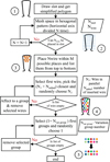 |
Fig. 1 General workflow for winding randomization. |
Afterward, groups need to be defined, as wires in the same group represent wires winded in parallel in the real motor. The variables N var group modify the way wires are grouped based on their relative distance: if the N var group is equal to zero, only the closest wires are selected to be part of a group, if the N var group is equal to the number of conductors, every conductor can be in any groups. For instance, in step 4 (Fig. 1), the N var group is equal to zero and groups of two wires are created, starting from the bottom center of the slot, the closest wire is grouped with its closest neighbor until all wires have a group. Finally, N added will randomly switch group order depending on the given value. This allows for variability in association and organization but does not change the conductors’ position. As shown in step 5 (Fig. 1), if N added is equal to one, an inversion of group order can be observed randomly. This process was designed to maximize the repartition within the slot, by creating such mesh, we are forcing all conductors to be separated in average by the maximal distance possible. Such a filling strategy is not entirely representative of the configuration found in real motors as the manufacturing process can spatially move any wire and is not the same throughout the motor length [20] but allows for variation studies in winding. Once this workflow has modified the overall winding, the following workflow will allow extracting HF impedance similar to [14–16].
3 FE simulations for impedance extraction
The geometry defined by the algorithm will be used to generate three FE models: two magnetic analyses and an electrostatic one using FEMM [21]. As the 2D nature of these tools cannot replicate the complexity of real electrical machines, hypotheses were taken. Indeed, contrary to [16], the studied motor end-windings lengths are not negligible, inducing a significant number of turn-to-turn capacitance and inductances in the overall motor winding.
3.1 Magnetic model for slot resistance and inductance
A section of the motor is drawn with a pole. As this PMSM only has one phase by slot, only two windings are represented to form the global induction loop Figure 2. All groups are excited one by one with a 1 A current to extract self and mutual impedances. For a given configuration of winding, all conductors in the same group are considered in parallel therefore the current is applied to all conductors leading to an overall impedance. By dividing the voltage drop, noted ΔV, by the total current I
i
flowing thought conductors in group i, resistance R and mutual-inductance as well as self-inductance L matrices are computed using equations (1) and (2):  (1)
(1)
 (2)
i: Group with 1 A imposed current, ω = 2πf.
(2)
i: Group with 1 A imposed current, ω = 2πf.
 |
Fig. 2 Slot impedance characterization with FEMM. |
For this simulation, insulation on the wire and in the slot is not represented as they behave very similarly to the air. Meshing is refined with regard to skin depth δ to extract coherent values: the outer edge of wire is fixed to δ/2. This process is illustrated in Figure 3 for three studied frequencies, 1 kHz, 1 MHz and 10 MHz, and a corresponding number of nodes is given in Table 1. Magnetic simulations are performed up to 10 MHz, resulting in more computationally intensive simulations at high frequency and in some cases instability in FEMM software as the mesh on wire circumferences is refined. Consequently, simulations do not exceed 10 MHz. This limitation is supposed to be due to the size of matrices exceeding the software capabilities. Finally, to consider the machine magnetization stack created by magnets, a simulation is performed beforehand without any current. The magnetic circuit characteristics are imported afterward using the frozen permeability feature of FEMM software.
 |
Fig. 3 Meshing refining for a 1 mm diameter copper wire at 1 kHz, 1 MHz, and 10 MHz. |
Node number for slot magnetic model with regard to frequency.
3.2 Capacitive model for turn-to-turn and turn-to-ground
Regarding capacitive computation, the process is similar to inductance and resistance estimation. All conductors in one group (shown by colors, Fig. 4) have their surfaces excited at 1 V, noted V
i
, in an electrostatic simulation while all others, as well as the slot border, are fixed at 0 V. Capacitance’s matrices C are therefore computed dividing surface charges q
j
on conductor j by V
i
as shown on equation (3). It is to be noted that in the case of i = j, the capacitance is in fact C
i-ground meaning the capacitance between the group i and the slot surface. (3)
i: Group with 1 V imposed excitation.
(3)
i: Group with 1 V imposed excitation.
 |
Fig. 4 Illustration of capacitive model with no enamel, featuring wire groups. |
3.3 Magnetic and electrostatic models for end-windings
The total length of the studied motor is composed of one-third of end-winding. Consequently, end-winding models were developed. However, using 2D FEM models, hypotheses need to be taken. The chosen approach uses an axisymmetric model: all conductors are kept in the same position as within the slot featured in Figure 4 and the distance to the revolution axis is half the distance between the two slots used by one coil, creating half a circle to generate a circularly ideal end-winding with no iron parts present. Coupling inductances between different phases are likewise considered negligible. Finally, these 2D approaches neglect end effects (local concentration of magnetic flux density in iron sheets at motor ends) and wire-to-iron stack capacitance. This approach is used to compute inductances and resistances as well as capacitances, similarly to their slot counterpart using equations (1), (2), and (3).
For the following results, the values chosen are: copper electrical conductivity, 58 MS/m, and relative permittivity equal to 1. M-36 Steel FEMM default material with a relative permittivity of 2.164. Wire insulation and slot insulation layer have both an electrical conductivity of 0 MS/m (like air) but a relative permittivity of 5. The stator considered in this work is around 50 mm lengthwise, with 100 mm and 150 mm for inner and outer diameters.
4 Spice circuit generation
All FEM simulations need to be integrated into an overall circuit to allow CM and DM impedance characterization. Figure 5 presents the electric model corresponding to one turn with associated nomenclature given in Table 2. For a motor with a single phase by slot, two main repeating units compose this circuit:
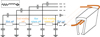 |
Fig. 5 Schematic spice used for circuit construction with matching 3D slot representation. |
Nomenclature used for lumped parameters.
4.1 Slot model with capacitive and inductive coupling
Ls and Rs components are respectively filled using R
ii
and L
ii
from equations (1) and (2); similarly, C
s is derived from equation (3). As one coil will go through two slots, this part needs to be repeated twice to get the desired behavior (Lsa – Lsr, Rsa – Rsr, and Csa – Csr). Finally, as this repeating unit is used for each turn in the electrical motor slot, mutual inductances between each group are implemented using equation (4) as Spice solver uses coupling factors and not mutual impedances. These coupling coefficients are named Ksa, Ksr, Kaa, and Kar matching the previous notation. (4)
(4)
4.2 Coupled real impedance generators
To add the real part of the coupled impedance, no passive components exist apart from the coupling factor in inductances. The real part of coupled impedances can be represented using behavioral voltage sources in the Spice simulator. The schematic described in [16] is not easily implementable in previously developed workflow therefore the equation (5) was used: (5)
(5)
One behavioral voltage source is used for each wire but the expression depends on the current within other groups. This source acts very similarly to the coupling coefficient for inductances and will simulate proximity effects generated by one wire group on other groups. Similarly, the coupling coefficient between inductances is placed for each conductor at every turn of the winding. The nomenclature adopted is Vsa, Vsr, Vaa, and Var.
4.3 End winding model
Similarly to their slot counterpart, resistor, inductance, coupling coefficient, and capacitances are used for both sides of the electrical machine (respectively Raa, Rar and Laa, Lar, Kaa, Kar and Caa, Car).
A resulting circuit is generated for each frequency point simulated and solved by LTSpice, capacitive couplings are considered constant at each frequency while resistance and inductance are highly impacted by skin and proximity effect. FEMM magnetic models are simulated at various frequencies and matrices are linearly interpolated to obtain in-between values. Laplace voltage-controlled generators were investigated similarly to [16] but due to the extensive number of expressions needed for a 80-turn electrical machine, the previous approach was preferred. Within this netlist, a voltage generator is placed either between ground and sa0 (node at the beginning of the coil) or between sa0 and arN (N being the number of turns) for respectively CM and DM impedance characterization. Combining these values and matching measurements on the existing motor will allow validation of the overall approach, similar to [14–16].
5 Studied configurations and HF trade-off
Three winding configurations are studied, depicted in Table 3. The aim is to compare three electrical machines considered equivalent from a mechanical standpoint but with different types of winding. The chosen enamel thickness matches the average IEC 06317 Grade 2, apart from S3 which is an estimated value to keep the same copper surface for all tested values. All these configurations are simulated with tools described before, allowing plotting of both CM and DM impedances. The following comparisons are based on a single coil and not on a full motor. On Figure 6, Table 3 configurations are simulated, configuration S1 is plotted in blue, S2 in orange, and S3 in red. Configurations S1-w/V to S3-w/V feature impedances computed without voltage-controlled sources representing proximity effects, differences with S1–S3 are discussed in Section 5.4. Finally, lumped parameters are computed in Table 4 for comparison.
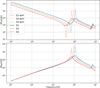 |
Fig. 6 CM and DM impedance of a simulated 80-turn coil with and without voltage-controlled sources using different winding. |
Studied PMSM winding configurations.
Nomenclature used for lumped parameters.
5.1 Common mode impedance
The common mode capacitance is the low-frequency capacitance that can be seen on the upper graph in Figure 6. It is computed with either Spice simulation or using a capacitance matrix trace. As more parallel conductors are used, more energy is stored between wires and the slot. This can be explained as the small wire tends to fill more of the space around the slot edge, increasing the capacitance between groups and the slot surface. Moreover, the enamel thickness does not decrease proportionally to the copper diameter, resulting in a bigger proportion of material with a high relative permittivity.
5.2 Differential mode inductance
Similarly to CM capacitance, DM inductances are estimated using the first part of curves on the lower graph in Figure 6. However, computing it from matrices can be difficult as coupled inductances impact the slope at the first order. This value does not vary significantly from configuration S1–S3.
5.3 AC resistance of coil
AC resistance is estimated as the sum of all resistances in series in the circuit Figure 6, or more simply the trace of matrix R, equation (2) at a given frequency. As this value is highly frequency dependent, a comparison between configurations is performed at 1 MHz. At this frequency, both skin and proximity effects highly impact the overall value. By computing the trace of the matrix resistance, it appears as if loss remains similar for every configuration. This result may appear counter-intuitive to the fact that reducing wire diameter (such as using Litz wires) reduces losses [22], but these observations are made at the motor working frequency and not at the high frequencies studied in this paper.
5.4 Real impedance coupled voltage generators
In the preliminary result, the real part of coupled impedances was neglected similarly to [14] as no behavioral voltage sources were used. As seen in Figure 6, such a circuit presented resonances with no damping (see S3-w/V compared to S3). In references [14, 15], the damping was not present in the curves obtained as no dielectric and iron losses were modeled. However, results presented in [16] have significant damping due to coupled real impedances but do not use any dielectric losses. Both authors in [14] and [23] noted a significant difference between their models and impedance measurements in particular on damping. No conclusion can be drawn to this question in the current study and further work is needed to conclude on the need to combine those aspects as no dielectric losses were taken into account in this paper. By comparing the curve from S1 to S3, no significant difference in damping can be observed between each configuration. The origin of such losses can be linked to induced current within other wires, coupled with proximity and skin effect. However as the frequency increases, the damping of resonances returns to the level of simulations without a voltage source, reducing the need to include the real part of coupled impedances in the spice netlist.
5.5 General remarks on impedance curves and resonances
Regarding common mode, the low-frequency capacitance seen on the various curves is driven by the capacitances of wires to slots, the first resonance is linked to both the line inductance (DM inductance in Tab. 4) and turn-to-turn capacitances [22]. As this inductance remains the same for all configurations and turn-to-turn capacitance is minimized due to the topology simulated, the first resonance is moved to lower frequencies whenever the CM capacitance is increased. The second resonance on CM impedance is more complex: as a difference in potential appears between each turn, a new association of capacitance is excited combining turn-to-turn and turn-to-slot capacitances. Following resonances are higher modes of the transmission line behavior of the system between the non-linear inductances of wires due to skin and proximity effects and all capacitances. The DM inductance computed in Table 4 drives DM impedances for the most part, skin and proximity effects change the value of self and mutual inductances, this results in a slight deviation from the expected 20 dB/decade slope, up until the first resonance with turn-to-turn capacitances change the behavior of the curve. Resonance frequencies match the CM impedance curve, resulting in similar behavior in both curves after the second and first resonance from CM and DM impedances respectively, implying that turn-to-turn capacitance is the main factor determining the first DM impedance resonance frequency in this winding configuration. A sensibility analysis was performed to validate the impact of such capacitance on impedance value Section 6.
6 Sensibility analysis to turn dispersion
The studied PMSM studied in this paper uses random wound: coils placed within the stator are mechanically formed either by hand or by an automated production line and placed in the stator. The exact place at which each conductor is placed is not known. General guidelines may be given to minimize overvoltage and differential tension between turns such as in [18, 19] but the exact whereabouts of each conductor are not known. To tackle this issue and understand the impact of such dispersion, a sensibility analysis was performed using only configuration S2 from Table 3. The studied configurations are regrouped in Table 5 and shown in Figure 7. The color of each wire in Figure 7 represents groups of wires in parallel. Configuration B1 is equivalent to Figure 4 S2 and features an ideal configuration where all wires are not mixed and turns with similar order remains adjacent to each other (the first turn is close to the second and third turn for instance) meanwhile configuration B2 and B3 degrade those factors, leading to B4 exhibiting the worst-case scenario. Impedance curves displayed in Figure 8 were obtained using the identical process as outlined before for configurations S1–S3.
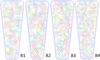 |
Fig. 7 B1 to B4 coil illustration with wire groups, without enamel. |
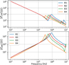 |
Fig. 8 CM and DM impedances with different winding configurations. |
Winding configurations for random wound.
6.1 Impedance modification due to variation in windings
Figure 8 displays both DM and CM impedance norms. B1 curves are equivalent to Figure 6 S2 simulations. With each configuration, as wires become increasingly shuffled within the slot, the first resonances are moved to a lower frequency. This phenomenon arises from the alteration of turn-to-turn capacitance between each configuration meanwhile the overall turn-to-slot capacitance is kept the same resulting in a low-frequency CM impedance value equal across all configurations. These observations provide further support for those made in [24]. Moreover, proximity effects can have a non-negligible impact on lower frequency inductances as shown by configuration B4 on DM impedance. Yet, for more realistic configurations (B1, B2, and B3), this disparity seems negligible on impedance value. Controlling the displacement of windings within the overall manufacturing process is therefore important to reduce insulation stress caused by dV/dt [18, 19] but also for reducing CM filtering devices.
6.2 Energy distribution in windings and impedance value over frequency
To visualize in more depth the contribution of each element (capacitances, inductances) to the overall impedance, the energy stored in the overall spice schematic is computed and classed into three categories (inductance, capacitance wires to ground, capacitance turn-to-turn) separated between slot and end-winding, resulting in a total of six categories. The accumulated stored energy is summed and shown at each frequency and normalized to compare every winding configuration. Figures 9 and 10 features winding B1 and B3 in CM and DM. Energy diagrams confirm that low-frequency CM impedance is driven by turn-to-slot capacitance. All configurations simulated share indeed the same value for CM capacitance in Figure 8 as every wire kept its respective place. This similarity remains until the first resonance, which features a different contribution depending on turn-to-turn capacitances. B1 impedance is driven by turn-to-slot capacitance meanwhile turn-to-turn capacitance makes the major contribution to B3 impedance after the first resonance. Similarities can be found in the DM impedance: low-frequency behavior is dictated by the inductance within the iron stack, as frequency increases, the contribution of turn-to-slot and turn-to-turn capacitance becomes more preponderant.
 |
Fig. 9 Energy ratio for CM impedance, configuration B1 and B3. |
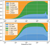 |
Fig. 10 Energy ratio for DM impedance, configuration B1 and B3. |
7 Experimental validation
To validate these findings, prototypes were developed to assess the influence of design decisions. A non-functional stator was assembled with nine coils. Three of each winding configuration (S1–S3) and mechanically assembled to facilitate consistent measurements as featured in Figure 11. These windings were measured using an impedance analyzer, between coils input and output and between coils input and stator iron stack to replicate DM and CM simulations respectively. The ground reference is the iron stack as the copper plate connected on each terminal block is electrically connected to iron sheets using copper tape. Experimental results are displayed in Figure 12 alongside simulations.
 |
Fig. 11 S1 to S3 windings assembled on a stator for validation. |
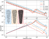 |
Fig. 12 Simulation and measurements for CM and DM impedance for S1 to S3 windings. |
As featured in Figure 12, the winding featuring the highest resonance frequencies was correctly identified and the evolution between measured configurations designed with different numbers of wires in parallel was accurately predicted, allowing designers to take into consideration ElectroMagnetic Compatibility (EMC) constraints at preliminary design stages. There is a distinct disparity between simulation and hand-on experiments, factors responsible for such differences is the placement of conductors: wire-to-slot capacitances are not fully represented as the filling algorithm tries to fill the slot uniformly but a denser pattern can appear toward some parts of the slot [20]. Furthermore, turn-to-turn capacitances in these simulations are minimized due to a wire grouping analogous to B1 Figure 7, it can indeed significantly reduce the frequency at which the first resonance can be seen as shown in Section 6 and [25].
8 Conclusion
In this paper, HF identification and simulation methodologies for various PMSM winding types were developed and tested. A geometry is generated with an associated winding, simulated using FEM, and equivalent impedance measurements are performed. This process is then used to evaluate the impact of wire in parallel and dispersion within slots. Finally, predictions are compared to measurements done on validation stators. Results show that increasing the number of wires in parallel for a given configuration of slots and turns carries a substantial risk of reducing the resonance frequency mainly driven by wire-to-slot capacitance. These phenomena will directly influence the system’s response to various regulations [10]. Further work is needed: dielectric losses need to be integrated to represent more accurately the resonance amplitudes and a physical model for wire placement and association would increase the accuracy of impedance values computed. Meanwhile, assessing the consequences of this behavior on the entire power drive and filtering devices will enlighten which trade-off needs to be made to improve global performances, with regard to regulation and system constraints. The robustness of such a tradeoff needs to be tested by introducing uncertainties in the winding that will represent the variations induced by fabrication processes. Finally, measurements and experiments allowed us to validate the evolution of impedances with regard to wires in parallel, despite differences mainly linked to random placement and displacement of wire within the slot.
Acknowledgments
This paper is part of the OCEANE Project led by IRT Saint Exupéry, Toulouse (France), which is sponsored by AIRBUS, LIEBHERR, SAFRAN, and the French National Research Agency (ANR) in collaboration with SATIE, TUD, DEEP, ICAM, and LAPLACE.
References
- Berger R., Nazukin M., Sachdeva N., Martinez N. (2017) Think: Act. Aircraft electrical propulsion – the next chapter of aviation? Roland Berger LTD, London, UK. [Google Scholar]
- Sathler H.H. (2021) Optimization of GaN-based series-parallel multilevel three-phase inverter for aircraft applications, PhD Thesis, Université Paris-Saclay, Gif-sur-Yvette, France, 284 p. [Google Scholar]
- Dos Santos V. (2019) Conducted electromagnetic emissions modeling in adjustable speed motor drive systems. Parametric studies and optimization of an inverter and filters under EMC constraints, PhD Thesis, INPT, Toulouse, France, 298 p. [Google Scholar]
- Hadden T., Jiang J., Bilgin B., Yang Y., Sathyan A., Dadkhah H., Emadi A. (2016) A review of shaft voltages and bearing currents in EV and HEV motors, in: IECON 2016 – 42nd Annual Conference of the IEEE Industrial Electronics Society, IEEE, pp. 1578–1583. https://doi.org/10.1109/IECON.2016.7793357. [CrossRef] [Google Scholar]
- Costello M.J. (1993) Shaft voltages and rotating machinery, IEEE Trans. Ind. Appl. 29, 2, 419–426. http://doi.org/10.1109/28.216553. [CrossRef] [Google Scholar]
- Plazenet T., Boileau T., Caironi C., Nahid-Mobarakeh B. (2018) A comprehensive study on shaft voltages and bearing currents in rotating machines, IEEE Trans. Ind. Appl. 54, 4, 3749–3759. http://doi.org/10.1109/TIA.2018.2818663. [CrossRef] [Google Scholar]
- Asefi M., Nazarzadeh J. (2017) Survey on high-frequency models of PWM electric drives for shaft voltage and bearing current analysis, IET Electr. Syst. Transp. 7, 3, 179–189. http://doi.org/10.1049/iet-est.2016.0051. [CrossRef] [Google Scholar]
- Shami U.T., Akagi H. (2010) Identification and discussion of the origin of a shaft end-to-end voltage in an inverter-driven motor, IEEE Trans. Power Electron. 25, 6, 1615–1625. http://doi.org/10.1109/TPEL.2009.2039582. [CrossRef] [Google Scholar]
- Morgan D., Mulhall B. (1995) A handbook for EMC testing and measurement. Measurement Science and Technology, 6, 5, IOP Publishing, Bristol, 600 p. [Google Scholar]
- Mariscotti A., Leonardo S. (2021) Review of models and measurement methods for compliance of electromagnetic emissions of electric machines and drives, Acta IMEKO 10, 2, 162–173. [CrossRef] [Google Scholar]
- Zhao D., Shen K., Liu W., Lang L., Liang P. (2019) A measurement-based wide-frequency model for aircraft wound-rotor synchronous machine, IEEE Trans. Magn. 55, 7, 8105408. https://doi.org/10.1109/TMAG.2019.2900616. [Google Scholar]
- Maki K., Funato H., Shao L. (2009) Motor modeling for EMC simulation by 3-D electromagnetic field analysis, IEEE International Electric Machines and Drives Conference, IEEE, pp. 103–108. https://doi.org/10.1109/IEMDC.2009.5075190. [Google Scholar]
- Gries M.A., Mirafzal B. (2008) Permanent magnet motor-drive frequency response characterization for transient phenomena and conducted EMI analysis, in: 2008 Twenty-Third Annual IEEE Applied Power Electronics Conference and Exposition, Austin, TX, USA, IEEE, pp. 1767–1775. https://doi.org/10.1109/APEC.2008.4522966 [Google Scholar]
- Boucenna N. (2014) HF common mode EMC modeling of AC three-phase motors, PhD Thesis, École normale supérieure de Cachan-ENS Cachan, Cachan, France, 166 p. [Google Scholar]
- Boucenna N., Costa F., Hlioui S., Revol B. (2016) Strategy for predictive modeling of the common-mode impedance of the stator coils in AC machines, IEEE Trans. Ind. Electron. 63, 12, 7360–7371. https://doi.org/10.1109/TIE.2016.2594052 [CrossRef] [Google Scholar]
- Ruiz-Sarrió J.E., Chauvicourt F., Gyselinck J., Martis C. (2021) High-frequency modelling of electrical machine windings using numerical methods, in: IEEE International Electric Machines & Drives Conference (IEMDC), IEEE, pp. 1–7. https://doi.org/10.1109/IEMDC47953.2021.9449561. [Google Scholar]
- Pastura M., Nuzzo S., Immovilli F., Toscani A., Rumi A., Cavallini A., Franceschini G., Barater D. (2021) Partial discharges in electrical machines for the more electric aircraft – Part I: A comprehensive modeling tool for the characterization of electric drives based on fast switching semiconductors, IEEE Access 9, 27109–27121. https://doi.org/10.1109/ACCESS.2021.3058083. [CrossRef] [Google Scholar]
- Mihaila V. (2011) New conception for AC machine’s stator winding minimizing dV/dt, PhD Thesis, Université d’Artois, Artois, 148 p. [Google Scholar]
- Mihaila V., Duchesne S., Roger D. (2011) A simulation method to predict the turn-to-turn voltage spikes in a PWM fed motor winding, IEEE Trans. Dielectr. Electr. Insul. 18, 5, 1609–1615. https://doi.org/10.1109/TDEI.2011.6032831. [CrossRef] [Google Scholar]
- Hoffmann A., Knebusch B., Stockbrügger J.O., Dittmann J., Ponick B. (2021) High-frequency analysis of electrical machines using probability density functions for an automated conductor placement of random-wound windings, in: IEEE International Electric Machines & Drives Conference (IEMDC), IEEE, pp. 1–2. https://doi.org/10.1109/IEMDC47953.2021.9449557. [Google Scholar]
- Meeker D. (2020) Finite element method magnetics user’s manual version 4.2, FEMM. 161 p. [Google Scholar]
- Pechlivanidou M.S.C., Kladas A.G. (2021) Litz wire strand shape impact analysis on AC losses of high-speed permanent magnet synchronous motors, in: 2021 IEEE Workshop on Electrical Machines Design, Control and Diagnosis (WEMDCD), IEEE, 95–100. https://doi.org/10.1109/WEMDCD51469.2021.9425656. [CrossRef] [Google Scholar]
- Ruiz Sarrio J.E., Chauvicourt F., Gyselinck J., Martis C. (2023) Impedance modelling oriented towards the early prediction of high-frequency response for permanent magnet synchronous machines, IEEE Trans. Ind. Electro. 70, 5, 4548–4557. https://doi.org/10.1109/TIE.2022.3189075. [CrossRef] [Google Scholar]
- Vostrov K., Pyrhönen J., Ahola J. (2019) The role of end-winding in building up parasitic capacitances in induction motors, in: 2019 IEEE International Electric Machines & Drives Conference (IEMDC), San Diego, CA, USA, IEEE, pp. 154–159. https://doi.org/10.1109/IEMDC.2019.8785238. [CrossRef] [Google Scholar]
- Ruiz-Sarrió J.E., Chauvicourt F., Martis C. (2022) Sensitivity analysis of a numerical high-frequency impedance model for rotating electrical machines, in: 2022 International Conference on Electrical Machines (ICEM), Valencia, Spain, 2022, IEEE, pp. 1260–1266. https://doi.org/10.1109/ICEM51905.2022.9910666. [CrossRef] [Google Scholar]
All Tables
All Figures
|
Fig. 1 General workflow for winding randomization. |
| In the text | |
|
Fig. 2 Slot impedance characterization with FEMM. |
| In the text | |
|
Fig. 3 Meshing refining for a 1 mm diameter copper wire at 1 kHz, 1 MHz, and 10 MHz. |
| In the text | |
|
Fig. 4 Illustration of capacitive model with no enamel, featuring wire groups. |
| In the text | |
|
Fig. 5 Schematic spice used for circuit construction with matching 3D slot representation. |
| In the text | |
|
Fig. 6 CM and DM impedance of a simulated 80-turn coil with and without voltage-controlled sources using different winding. |
| In the text | |
|
Fig. 7 B1 to B4 coil illustration with wire groups, without enamel. |
| In the text | |
|
Fig. 8 CM and DM impedances with different winding configurations. |
| In the text | |
|
Fig. 9 Energy ratio for CM impedance, configuration B1 and B3. |
| In the text | |
|
Fig. 10 Energy ratio for DM impedance, configuration B1 and B3. |
| In the text | |
|
Fig. 11 S1 to S3 windings assembled on a stator for validation. |
| In the text | |
|
Fig. 12 Simulation and measurements for CM and DM impedance for S1 to S3 windings. |
| In the text | |
Current usage metrics show cumulative count of Article Views (full-text article views including HTML views, PDF and ePub downloads, according to the available data) and Abstracts Views on Vision4Press platform.
Data correspond to usage on the plateform after 2015. The current usage metrics is available 48-96 hours after online publication and is updated daily on week days.
Initial download of the metrics may take a while.