


| Issue |
Sci. Tech. Energ. Transition
Volume 81, 2026
Enabling Technologies for the Integration of Electrical Systems in Sustainable Energy Conversion
|
|
|---|---|---|
| Article Number | 16 | |
| Number of page(s) | 12 | |
| DOI | https://doi.org/10.2516/stet/2026014 | |
| Published online | 05 May 2026 | |
Regular Article
Evaluation of power losses and their impact on battery life in AC, DC, and hybrid microgrids
1
Université de Tunis El Manar, LSE-LR11 ES15, ENIT, BP, 37 le belvédère 1002, Tunis, Tunisia
2
Université de Carthage, IPEIN, Université de Tunis El Manar, LSE-LR11 ES15, ENIT, BP, 37 le belvédère 1002, Tunis, Tunisia
3
Université de Tunis, ENSIT, Université de Tunis El Manar, LSE-LR11 ES15,ENIT, BP 37 le belvedére 1002, Tunis, Tunisia
* Corresponding author: This email address is being protected from spambots. You need JavaScript enabled to view it.
Received:
27
March
2025
Accepted:
10
March
2026
Abstract
Microgrids (MGs) are being deployed more extensively worldwide, as they represent the most viable solution for expanding energy access in energy-poor countries. Power loss is a fundamental factor to consider, as it directly impacts the overall efficiency and cost-effectiveness of the system. Power loss occurs in various microgrid components, including lines, converters, and power electronic devices. In the first stage, transmission line voltage droop and power losses were determined for different microgrid topologies. The second stage involved analyzing power losses across all converters (specifically switching and conduction losses) to determine the operational efficiency of each unit. The total power loss summation allowed for an evaluation of global microgrid efficiency, facilitating the identification of the optimal configuration. Furthermore, battery State of Charge (SOC) and Depth of Discharge (DOD) were analyzed across the different topologies, accounting for both ideal and loss-affected scenarios. The findings indicate that DC microgrids maintain a higher SOC, whereas AC configurations lead to a lower SOC; these variations in DOD directly impact the projected battery cycle life. In addition to MATLAB/Simulink simulations, HOMER Pro software was employed to perform design optimization and evaluate energy management strategies. This provided a comparative analysis of the economic feasibility across the proposed microgrid topologies.
Key words: Microgrid / System losses / Voltage droop / Power efficiency / SOC / DOD
© The Author(s), published by EDP Sciences, 2026
 This is an Open Access article distributed under the terms of the Creative Commons Attribution License (https://creativecommons.org/licenses/by/4.0), which permits unrestricted use, distribution, and reproduction in any medium, provided the original work is properly cited.
1 Introduction: The concept of microgrid
With the development of single- and three-phase transformers, alternating current could be transmitted over long distances at high voltages. Consequently, the lower cost of AC power distribution predominated, while DC systems persisted only in certain urban areas throughout the 20th century [1].
More recently, DC microgrids have become viable; the transition from AC grids to a distributed power world is expected to be rapid, driven by significant advantages in cost, efficiency, reliability, and system resilience [2, 3]. According to the International Renewable Energy Agency (IRENA), AC microgrids represented 95% of the global market in 2021, while DC microgrids held the remaining 5%. Several factors contribute to the dominance of AC systems, notably the widespread availability and relatively low cost of AC components. However, DC microgrids are gaining traction due to their inherent advantages, such as higher efficiency, greater flexibility, and improved reliability. As the cost of DC power conversion technology continues to decrease, a significant shift toward DC microgrid architectures is expected in the coming years [4].
Hybrid microgrids are currently the least deployed worldwide; however, they are under active development as they combine the advantages of both AC and DC systems. They offer superior resilience against extreme events, such as earthquakes and short circuits. In some cases, renewable energy systems are grid-connected for continuous energy injection. However, this topology faces security constraints due to the fluctuations in both consumption and renewable power generation. To mitigate these negative impacts, many countries have adopted energy tariffs that discourage permanent injection, instead favoring self-consumption.
Following this global trend toward photovoltaic (PV) energy, Tunisia has implemented specific programs to exploit its solar potential. Initially, the Tunisian PV market focused on rural electrification for populations unable to connect to the STEG (Tunisian Company of Electricity and Gas) network due to economic constraints [5]. Currently, approximately 13,000 rural households are equipped with 100 W kits for lighting and audiovisual needs. In total, about 1.4 MW was installed between 2000 and 2010, with an average annual growth rate of 7% [6].
In 2012, only 70 kW were installed, reflecting the limited remaining potential for this specific market, as 99.6% of the Tunisian population is already connected to the STEG grid. However, the concepts of self-production and self-consumption have gained significant momentum internationally. Consequently, the Tunisian regulatory framework for low- and medium-power photovoltaic installations has evolved remarkably, and administrative procedures have been streamlined [7].
To ensure power balance and optimize overall operation, a precise understanding of microgrid dynamics is essential. Previous research has demonstrated that accurate predictions of PV generation and load demand significantly influence optimization outcomes [8, 9]. This study focuses on evaluating power losses in both transmission lines and converters to minimize energy waste and optimize power flow. Furthermore, battery performance is a critical factor in microgrid efficiency and sustainability. Given that battery longevity is highly sensitive to the State of Charge (SOC) and Depth of Discharge (DOD), this study evaluates these parameters across various microgrid architectures. This analysis aims to pinpoint the optimal configuration for maximizing battery life while ensuring robust system reliability.
2 Microgrids classifications
Microgrids typically incorporate photovoltaic arrays, wind turbines, and battery storage to mitigate the intermittency of renewable generation. These systems operate in two distinct configurations: grid-tied, where interaction with the utility network enhances economic performance through bidirectional energy flow; and standalone, where the microgrid decouples from the main grid during outages to maintain power quality and reliability for essential services.
Depending on their coupling architecture, microgrids are categorized as AC, DC, or hybrid types. AC configurations typically utilize single-phase or three-phase buses, whereas DC microgrids are implemented through unipolar, bipolar, or ring topologies. Given the complexity of these structural variations, determining the most suitable architecture requires a multi-criteria analysis. This study focuses specifically on overall system efficiency as the decisive metric for benchmarking these configurations [10–12].
The efficiency of a microgrid depends on several factors, including power losses in transmission lines, converters, and energy sources. By considering these losses, the management system can be optimized, leading to improved overall performance and reliability.
2.1 AC microgrids
All energy sources supply power to the loads through an AC bus. Photovoltaic (PV) systems and batteries, classified as DC energy sources, require a DC/AC inverter to connect to the AC bus. In contrast, AC generators such as wind turbines and diesel generators can be directly linked to the AC bus Figure 1.
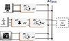 |
Figure 1 AC microgrid configuration. |
2.2 DC microgrids
All energy sources supply power to the loads through a DC bus. Photovoltaic (PV) systems and batteries, being DC sources, connect directly to the DC bus without needing conversion. However, AC generators such as wind turbines and diesel generators require an AC/DC converter to integrate into the system. This topology uses fewer converters, which can reduce costs. A typical topology DC microgrid is shown in Figure 2.
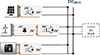 |
Figure 2 DC microgrid configuration. |
The control of converters in a DC microgrid is simpler compared to an AC microgrid, as there is no need to manage reactive power flow. Additionally, DC microgrid operation is easier because it does not require phase and frequency regulation.
2.3 Hybrid microgrids
Hybrid microgrids combine AC and DC networks using bidirectional converters. This design improves power quality by reducing unnecessary conversion stages. AC sources and loads connect to the AC bus, while DC components connect to the DC bus. The battery storage can be placed on either side, which makes energy management more flexible. Although this system is more complex and can increase power losses because of the extra converters, it has one major advantage: it keeps running even if a short circuit occurs on one of the buses [4, 13, 14].
The diagram of a hybrid microgrid is illustrated in Figure 3.
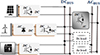 |
Figure 3 Hybrid microgrid configuration. |
2.4 Microgrid power sharing
Three types of power (source, load, and battery) work together in a coordinated way to ensure the microgrid operates efficiently, remains resilient, and can effectively supervise renewable energy variability, load changes, and power reliability [15].
PV power system (Ppv) was provided by multiplying the product of total efficiency, the panel’s area APV (m2) and the solar irradiance Ir (W/m2) [16]. (1)
(1)
The power produced by the wind turbine was obtained by applying the following equation [17, 18]. (2)
(2)
The state of charge of the battery power is determined by (3)
(3)
Power losses in microgrid lines depend on the number of wires and the voltage level. Usually, more wires mean higher losses. While AC and DC microgrids use only two wires, hybrid microgrids require four. Similarly, the more converters a system has, the higher the power losses will be. By looking at the microgrid designs in Figures 1–3, we can optimize the layout to use fewer converters and improve energy efficiency.
2.5 Line power losses
The internal resistance of power sources can vary depending on the type of power source and its operating conditions, and the impedance of the lines connecting the power sources to the load can also contribute to voltage droop. Again, the impedance of a line depends on its length, material, and cross-sectional area. Finally, the current flowing through the microgrid influences the voltage droop [15]. (4)
(4) (5)
(5) (6)
(6) (7)
(7)
 ; L represents the line length, S designates the cable cross-section, and ρ = 0.025 Ω·mm2/m is the resistivity of copper.
 ; λ = 0.08 mῼ/m is reactance of the copper line, is the impedance line phase factor.
The power loss in line equal to; (8)
(8) (9)
(9)
In a DC system with a constant power load, the voltage droop depends only on the bus voltage level. This is different from an AC system, where the voltage droop is affected by the bus voltage and the load’s phase factor. (10)
(10)
The variation of this ratio is depicted in Figure 4.
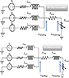 |
Figure 4 Ratio evolution as a function of phase |

A DC microgrid offers greater benefits by reducing transmission losses compared to an AC microgrid when both have the same peak voltage, as shown in equation (26) [19].
The theveinin model of hybrid microgrid combined the last two AC and DC models and it’s presented by Figure 5.
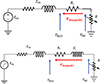 |
Figure 5 Hybrid microgrid Thevenin model. |
In the hybrid microgrid case, the voltage droop and line power loss are equal to the superposition of AC branch and DC branch.
 (11)
(11)
The hybrid line power loss equation can be rewritten as follows:
α, β are coefficients that represent the relative contributions of AC and DC power loss to the overall hybrid line power loss. (12)
(12)
The evolution of the ratio is shown Figure 6.
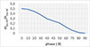 |
Figure 6 Evolution of ratio with different phase factor and different load repartition. |
This ratio shows that line power loss in hybrid microgrid is less than of an AC microgrid.
If α = 1, the hybrid line is essentially AC line. So, the line power loss will be increase to the maximum value.
If α = 0, the hybrid line is essentially a DC line and the line power loss will be decrease to the minimum value.
If α and β are both non-zero, then the hybrid line combines the advantages of both AC and DC lines.
2.6 Microgrids converters power loss
The power generation system integrates solar panels, wind turbines, and a battery bank to provide a sustainable energy source. To ensure efficient power management and distribution, several converter stages are utilized.
Within the DC microgrid, a boost converter interfaces with the solar panels to step up the voltage for system integration. The wind turbine utilizes a three-phase rectifier coupled with a second boost converter to facilitate energy sharing. Furthermore, a bidirectional converter is connected to the battery bank, allowing for seamless energy storage and demand-side management.
In the AC microgrid configuration, an inverter is integrated into each source to convert the DC power generated by the solar panels and wind turbines into AC power. This conversion ensures seamless compatibility with AC loads. Furthermore, the deployment of individual inverters at each source enhances the flexibility and adaptability of the microgrid (Fig. 1).
To achieve a more simplified and cost-effective architecture, a hybrid microgrid design is proposed where a central inverter is integrated into the DC bus. This configuration utilizes two distinct bus voltages to efficiently accommodate both types of loads (Fig. 3). Finally, a comprehensive analysis of the power losses associated with each converter stage is conducted to evaluate overall system efficiency.
3 Technical analysis
Power losses in a microgrid reduce overall efficiency and the amount of usable energy delivered to consumers. The resulting heat can damage components and raise maintenance expenses. Unchecked, these losses threaten grid stability. Therefore, the preceding part focused on modeling different microgrid topologies to assess voltage droop and power loss performance.
3.1 Model of AC and DC microgrids
Voltage droop is a phenomenon where the voltage at a specific point in a microgrid decreases as the load current increases. This droop can lead to several negative consequences, including reduced power quality, increased power losses, and decreased system stability.
The circuit diagram is designed with the assumption that all power supplies operate as constant voltage sources. In a DC microgrid, Voltage is regulated by a DC/DC converter, operating as an ideal buck or boost stage to step the voltage up or down [20]. In contrast, an AC microgrid utilizes a DC/AC converter (inverter) for voltage conversion, as illustrated in Figure 7.
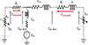 |
Figure 7 Electrical schema for DC and AC microgrid. |
The Thevenin voltage source and Thevenin impedance will be equal to: (13)
(13) (14)
(14)
The AC and DC microgrid Thevenin model is presented in Figure 8.
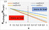 |
Figure 8 DC and AC microgrid Thevenin model. |
3.2 Converters model
The efficiency of converters integrated into a microgrid can be affected by various factors, leading to variations in performance even under consistent operating conditions. Several key factors contribute to power loss in DC/DC converters:
Switching losses : These losses arise from the switching process within the converter as the transistors repeatedly turn on and off. The switching frequency, as well as the voltage and current levels across the transistors, significantly impact the magnitude of these losses.
Conduction losses : These losses result from the resistance of the internal components of the converter, such as transistors, inductors, and capacitors. The current flowing through these components generates heat, which dissipates as power loss [21].
power losses in the boost converter (Fig. 9)
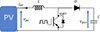 |
Figure 9 PV boost converter electrical schema. |
The Inductor conduction loss is calculated by:

The power loss model of this converter is: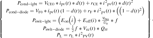 (15)
(15)
The energy efficiency of the PV boost converter is: (16)
(16)
By the same means the power loss in the boost converter associated with the wind power is equal to:
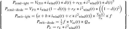 (17)
(17)
The energy efficiency of the wind boost converter is: (18)
(18)
Power loss in the battery converter
The Bidirectional DC/DC Converter (Fig. 10) manages battery energy flow by switching between two modes:
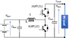 |
Figure 10 Battery converter electrical schema. |
The Buck Mode (Charging): Steps down DC bus voltage to charge the battery when production exceeds demand. The Boost Mode (Discharging): Steps up battery voltage to support the load when renewable production is low.
The efficiency of this converter is calculated by equation (19). (19)
(19)
Power losses in the inverter
The inverter is used in AC and Hybrid microgrid, the electrical schema is shown in Figure 11.
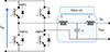 |
Figure 11 Inverter electrical schema. |
The total power loss in the switch is expressed as; (20)
(20)
The power loss model of inverter is given by equation (21):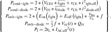 (21)
(21)
The energy efficiency of the inverter is: (22)
(22)
Three-phase rectifier power losses
For high-power needs, three-phase bridge rectifiers are commonly used. This converter connects directly to the wind turbine. Figure 12 shows the electrical circuit.
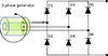 |
Figure 12 Three-phase Rectifier schema. |
The conduction power in all diodes is; (23)
(23)
With  the internal diode resistance, and ID is the current in the diode.
The rectifier efficiency will be obtained by equation (24) [22, 23]. (24)
(24)
3.3 Simulation and results interpretation
The simulation parameters are derived in Table 1.
Simulation parameters.
The source profile and load profile are shown in the following figure.
In this simulation, the load is kept constant at 1.5 kW to ensure a stable power line, while the PV and wind power profiles vary to introduce multiple input power sources. The PV power exhibits faster dynamics (0.05 s) compared to the wind turbine (1.5 s), leading to different transient behaviors. The total renewable power reaches its maximum between 2 s and 4 s, while the minimum generated power occurs between 1 s and 1.5 s. These fluctuations directly impact converter losses, influencing both efficiency and thermal performance within the microgrid Figure 13.
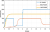 |
Figure 13 Pv, wind and load profiles. |
Figure 14 represents the sending voltage for both DC and AC microgrids, as well as the receiving voltage at the load for both cases. For a load of 1.5 kW, the current in the line causes a droop voltage of 2 V in the DC bus and 5 V in the AC bus. The advantage of the DC droop voltage is due to the absence of line reactance, which results in a more efficient and stable voltage Figure 14.
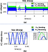 |
Figure 14 Droop voltage of AC and DC microgrid. |
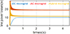 |
Figure 15 Line power losses progression. |
In Figure 14, the AC microgrid exhibits the highest power losses of approximately 19 W, attributed to resistive and reactive losses in AC transmission. Conversely, the DC microgrid shows the lowest losses, stabilizing around 10 w, due to the absence of reactive power losses. The hybrid microgrid, incorporating both AC and DC elements, demonstrates intermediate losses of approximately 11 W, reflecting a balance between the benefits of DC efficiency and the inherent losses of AC components.
It’s crucial to note that the line power losses are directly related to the current flowing through the conductors, which, under a fixed load, remain relatively constant in the steady-state. However, the losses associated with the converters of the hybrid system are more nuanced. These converter losses are significantly influenced by the current sharing between the generation sources and the energy storage branches. Specifically, the maximum converter power losses are observed between 2 and 4 s, likely due to increased current flow resulting from source variations. Conversely, the minimum converter power losses occur between 1 and 1.5 s, indicating that the cause is the decreased current from the sources Figure 16.
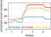 |
Figure 16 Converters power losses evolution. |
Figure 17, shows that the DC-MG efficiency can reach a maximum value of 95% and decrease to 93%. This can be due to the renewable power source. On the other hand, the AC microgrid and hybrid microgrid efficiencies are respectively 90% and 92%.
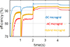 |
Figure 17 Microgrid efficiency. |
The DC microgrid (DC-MG) achieves a maximum efficiency of 95%, which is the highest among the systems. The AC microgrid has an efficiency of 90%, while the hybrid microgrid performs at 93% efficiency. This shows that the DC-MG performs best under stable conditions, while the AC and hybrid microgrids are more affected by fluctuations in the power supply.
Additionally, the hybrid microgrid has variable efficiency depending on the type of load and whether connected to the DC or AC buses. The efficiency of the hybrid system can change based on the load conditions, with different performance characteristics for DC and AC loads.
Overall, the DC microgrid outperforms the other systems in this comparison due to its higher efficiency and better performance under stable conditions. These results encourage further study of the impact of State of Charge (SOC) and Depth of Discharge (DOD) of the battery in the next section.
4 Battery cycle life for AC, DC, hybrid microgrid
The battery life cycle refers to the number of charge and discharge cycles a battery can complete before its capacity significantly declines. Two critical factors influencing battery performance over time are the State of Charge (SOC) and the Depth of Discharge (DOD) [24, 25].
4.1 Impact on battery SOC
In this study, the analysis of battery performance and SOC variations is conducted over a one-month period using HOMER software.
Table 2 presents the parameters for a hybrid power station (Solar/Wind) operating over a one-month period with a variable 1.5 kW peak load.
Input parameters for hybrid system simulation (month: August).
The load profile remains the same across all three microgrid configurations (DC, AC, and Hybrid). In a DC Microgrid, the load is directly supplied by the DC system; in an AC Microgrid, the load is adapted for AC supply; and in a Hybrid Microgrid, the load is split between the DC and AC subsystems, with the sum of both loads equal to the original load, ensuring energy balance Figures 18 and 19.
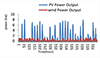 |
Figure 18 Sources power generated. |
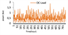 |
Figure 19 Load power demand. |
The energy management systems are responsible for coordinating power distribution among all the components of the microgrid. It operates in both buck and boost modes to meet the load demand and charge the battery.
The ideal SOC of the battery can be estimated as follows: [26, 27]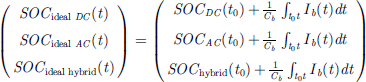 (25)
(25)
The real SOC of the battery is determined by;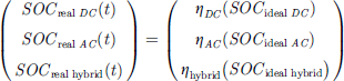 (26)
(26)
With:
 : represents the global efficiency of the DC microgrid
 : represents the global efficiency of the DC microgrid
η hybrid: represents the global efficiency of the DC microgrid
The simulation result using Homer software is presented by the following figures (Figs. 20–22).
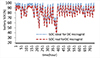 |
Figure 20 Ideal and real battery SOC for DC microgrid. |
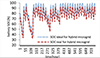 |
Figure 21 Ideal and real battery SOC for hybrid microgrid. |
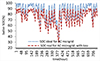 |
Figure 22 Ideal and real battery SOC AC microgrid. |
The simulation results show variations in the State of Charge (SOC) of the battery across different microgrid topologies, both with and without power loss consideration. The DC microgrid (Fig. 1) exhibits the lowest SOC, while the AC microgrid (Fig. 2) shows the highest SOC, and the hybrid microgrid (Fig. 3) presents an intermediate SOC level. This variation directly impacts the Depth of Discharge (DOD) of the battery, where a lower SOC leads to a higher DOD, potentially accelerating battery aging and reducing its lifespan, whereas a higher SOC results in a lower DOD, improving battery durability. In the next figure, the average Depth of Discharge will be calculated for each case to further analyze the battery performance under different microgrid configurations.
4.2 Impact on battery DOD
Depth of Discharge (DOD) is influenced by the topology of the microgrid. For each type of microgrid (DC, AC, or hybrid), the DOD is determined based on the State of Charge (SOC) of the battery. The DOD is affected by the specific power conversion and transmission characteristics of each system, which influence how energy is stored, converted, and discharged [28].
The following equation represents the relationship for DOD in terms of SOC [29].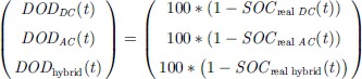 (27)
(27)
The result of the DOD from the previous simulation is presented in Figure 23.
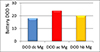 |
Figure 23 DOD battery evolution. |
The Depth of Discharge (DOD) varies significantly with microgrid architecture, which will affect the battery life cycle. DC microgrids show the lowest DOD at 18%, indicating the most efficient battery discharge management and likely the longest lifespan. AC microgrids have the highest DOD at 24%, suggesting greater discharge and potentially a shorter battery life. Hybrid microgrids fall in between with a DOD of around 20%, reflecting a mix of AC and DC characteristics. Overall, DC microgrids offer the best battery lifespan preservation due to their superior discharge management. Figure 24, illustrates the battery life cycle for each case.
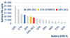 |
Figure 24 Battery life cycle. |
The graph demonstrates that Battery Life Cycle Number varies with microgrid architecture due to differences in Depth of Discharge (DOD%). In a DC microgrid, where DOD is lowest (~18%), the battery achieves the highest life cycle number at Ndc = 12,000 cycles. In contrast, the AC microgrid, with the highest DOD (~24%), results in a reduced cycle life of Nac = 9,000 cycles. The Hybrid microgrid, with an intermediate DOD (~20%), maintains a balanced life cycle of Nhybrid = 10,000 cycles. This confirms that lower DOD leads to extended battery lifespan, making DC microgrids the most efficient for long-term battery performance.
5 Experimental study
The experimental step is designed to determine the voltage droop and power loss in a copper transmission line that is 100 m long with a cross-section of 1.5 mm2 (Fig. 25).
 |
Figure 25 Experimentation of DC microgrid. |
The following experiments analyze how bus voltage evolves with changes in load current. Two voltage levels are considered: very low voltage (VLV) and low voltage (LV).
For VLV buses (24 V, 48 V), a higher load current significantly affects stability, as shown in Figure 26. The voltage droop can reach up to 30%, leading to poor transmission efficiency, which tends to be around 70%. In this case, implementing a droop control method can help regulate the voltage level.
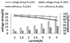 |
Figure 26 VLV .Voltage droop. |
In the case of LV buses (300 V and 600 V), system performance improves, with the voltage droop limited to only 1%. As a result, the transmission efficiency reaches up to 98%, as observed in Figure 27.
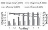 |
Figure 27 LV. Voltage droop. |
6 Conclusion
This paper presents an innovative approach for assessing the technical benefits of AC, DC, and hybrid microgrids. The framework reveals that DC microgrids can achieve superior system efficiency with the same distribution infrastructure as AC and hybrid microgrids. To determine the line losses, the authors develop Thevenin models for each microgrid type. Since transmission line losses depend on the load current, it is essential to have the same load for each distribution. The results show that the DC line losses are significantly lower than the AC and hybrid transmission losses. This part is validated by an experimental study for different bus types and voltage levels (300 V DC, 220 V AC, 12 V, 24 V, 48 V, 300 V DC, 600 V DC). In addition, the authors examine the losses in power converters, with the DC architecture utilizing the minimum number of converters, resulting in the lowest converter losses and further improving overall system efficiency.
The study also addresses the impact of these power losses on the state of charge (SOC) and depth of discharge (DOD) of the battery. The reduced line and converter losses in DC microgrids lead to more efficient energy storage and management. As a result, the DC microgrid configuration results in lower DOD and slower SOC depletion, which translates to longer battery life. The findings show that DC microgrids provide the most effective energy storage solution, with a longer battery lifespan due to reduced losses, making it the optimal choice for sustainable and efficient energy management.
References
- Guerrero J. M., Vasquez J. C., Gomez-Arias J. T., Luna M. (2023) Toward a resilient future: A review of DC microgrid architectures for enhanced reliability and stability, Sustain. Energy Technol. Assess. 55, 143–158. [Google Scholar]
- Al-Saffar A. H., Al-Saffar A. A. M., Al-Saffar H. A. (2023) Cost-effectiveness analysis of AC vs DC microgrids for rural electrification in developing countries, Energy Rep. 9, 471–480. [Google Scholar]
- Mousavi S.D., Golshani M.A., Savadkoohi M. (2023) Hybrid AC/DC microgrids: A promising solution for integrating high-penetration renewables, Renew. Energy 232, 1004–1017. [Google Scholar]
- Opiyo N.N. (2019) A comparison of DC-versus AC-based minigrids for cost-effective electrification of rural developing communities, Energy Rep., 398–408. [Google Scholar]
- Agence Nationale pour la Maîtrise de l'Énergie (ANME) (2015) Plan Solaire Tunisien, 2030. [Google Scholar]
- Commission de Régulation de l'Électricité et du Gaz (CREG) (2023) Cadre réglementaire relatif au système de photovoltaïque raccordé au réseau et à l'autoconsommation. [Google Scholar]
- Bellil H., Ben Amor B., Elghouch E.M. (2016) Renewable energy policy design and its effects on the PV market development in Tunisia, Environ. Prog. Sustain. Energy 35(2), 555–562. [Google Scholar]
- Ben Salah S., Alaya M.B., Ben Romdhane M. (2018) Barriers and opportunities for photovoltaic off-grid systems in Tunisia, Int. J. Green Energy 15(4), 346–357. [Google Scholar]
- Hamdi-Cherif S., Kara I., Boujelben F. (2019) Evolution of the Algerian and Tunisian regulatory frameworks for small-scale photovoltaic installations, Energy Proc. 157, 833–842. [Google Scholar]
- Hirsh A., Parag Y., Guerrero J. (2018) Microgrids: A review of technologies key drivers, and outstanding issues, Renew. Sust. Energ. Rev. 90, 402–411. [Google Scholar]
- Dagar A., Gupta P., Niranjan V. (2021) Microgrid protection: A comprehensive review, Renew. Sust. Energ. Rev. 149, 111401. [Google Scholar]
- Mohamad A.M.E.I., Yari M. (2019) Investigation and assessment of stabilization solutions for DC microgrid with dynamic loads, IEEE Trans. Smart Grid 10, 5735–5747. [Google Scholar]
- Planas E., Andreu J., Gárate J.I., Ibarra E. (2015) AC and DC technology in microgrids: A review, Renew. Sust. Energ. Rev. 43, 726–749. [Google Scholar]
- Ullah S. et al. (2020) Assessment of technical and financial benefits of AC and DC microgrids based on solar photovoltaic, electrical engineering journal, Springer. [Google Scholar]
- Mohammed N., Callegaro L., Ciobotaru M., Guerrero J.M. (2023) Accurate power sharing for islanded DC microgrids considering mismatched feeder resistances, Appl. Energy, 340, 121060. [Google Scholar]
- Saranya A., Swarup K.S. (2017) Sizing of solar DC microgrid for sustainable off-grid communities, in Conference on Sustainable Green Buildings and Communities (SGBC). [Google Scholar]
- Fakhar A., Haidar A.M.A., Ahmed M.M., Rahman A.K. (2018) Sustainable energy management design for Bario microgrid in Sarawak, Malaysia, in IEEE 7th International Conference on Power Energy. [Google Scholar]
- Khlifi F., Cherif H., Belhadj J. (2021) Environmental and economic optimization and sizing of a micro-grid with battery storage for an industrial application, Energies, 14, 5913. [Google Scholar]
- Starke M., Tolbert L.M. (2008) AC vs. DC distribution: a loss comparison, in IEEE PES Transmission and Distribution Conference and Exposition. [Google Scholar]
- Chang F., Cui X., Wang M. (2021) Potential-based large-signal stability analysis in DC power grids with multiple constant power loads, Access J. Power Energy 99, 1–1. [Google Scholar]
- Khaterchi H., Regaya C.B., Jeridi A., Zaafouri A. (2025) Innovative hybrid war strategy optimization with incremental conductance for maximum power point tracking in partially shaded photovoltaic systems, Power Electron. Drives, 10. [Google Scholar]
- Lee Y.S., Chow M.H.L. (2018) Diode rectifiers, power electronics handbook (fourth edition), pp. 177–208. [Google Scholar]
- Buchert K., Fuchs F.W. (2015) Power losses of three-phase rectifier topologies in small wind Turbines, in Proceedings of PCIM Europe, Germany. [Google Scholar]
- Ennassiri Y., de-Simón-Martín M., Bracco S., Robba M. (2024) Energy management system for polygeneration microgrids, including battery degradation and curtailment costs, Sensors, 24(22), 7122. [Google Scholar]
- Vaka S.S.K.R., Kumari M.S. (2024) Optimal Sizing of Battery Energy Storage Systems Considering Degradation Effect for Operating and Electricity Cost Minimization in Microgrids, Energy Technol., 12(1), 2300704. [Google Scholar]
- Albasheri M.A., Bouchhida O., Soufi Y., Cherifi A. (2024) enhanced supervisor energy management technique of DC microgrid-Based PV/Wind/Battery/SC, Electr. Eng. 107, 2285–2296. [Google Scholar]
- Yang T., Song D. (2024) Design of Optimal Wavelet-Based Energy Management for Hybrid Energy Storage Systems in DC-Microgrids to Increase the Battery Lifetime, Multiscale Multidiscip. Model. Exp. Des., 7, 3243–3252. [Google Scholar]
- Amiri M.H.N., Annaz F., De Oliveira M., Gueniat F. (2024) Resilient Islanded Microgrid Battery Energy Management Considering the Life of Battery, arXiv preprint arXiv:2407.10278. [Google Scholar]
- Escobar E.D., Betancur D., Isaac I.A. (2024) Optimal Power and Battery Storage Dispatch Architecture for Microgrids: Implementation in a Campus Microgrid, Smart Grids Sustain. Energy, 9, 27. [Google Scholar]
All Tables
All Figures
|
Figure 1 AC microgrid configuration. |
| In the text | |
|
Figure 2 DC microgrid configuration. |
| In the text | |
|
Figure 3 Hybrid microgrid configuration. |
| In the text | |
|
Figure 4 Ratio evolution as a function of phase |
| In the text | |
|
Figure 5 Hybrid microgrid Thevenin model. |
| In the text | |
|
Figure 6 Evolution of ratio with different phase factor and different load repartition. |
| In the text | |
|
Figure 7 Electrical schema for DC and AC microgrid. |
| In the text | |
|
Figure 8 DC and AC microgrid Thevenin model. |
| In the text | |
|
Figure 9 PV boost converter electrical schema. |
| In the text | |
|
Figure 10 Battery converter electrical schema. |
| In the text | |
|
Figure 11 Inverter electrical schema. |
| In the text | |
|
Figure 12 Three-phase Rectifier schema. |
| In the text | |
|
Figure 13 Pv, wind and load profiles. |
| In the text | |
|
Figure 14 Droop voltage of AC and DC microgrid. |
| In the text | |
|
Figure 15 Line power losses progression. |
| In the text | |
|
Figure 16 Converters power losses evolution. |
| In the text | |
|
Figure 17 Microgrid efficiency. |
| In the text | |
|
Figure 18 Sources power generated. |
| In the text | |
|
Figure 19 Load power demand. |
| In the text | |
|
Figure 20 Ideal and real battery SOC for DC microgrid. |
| In the text | |
|
Figure 21 Ideal and real battery SOC for hybrid microgrid. |
| In the text | |
|
Figure 22 Ideal and real battery SOC AC microgrid. |
| In the text | |
|
Figure 23 DOD battery evolution. |
| In the text | |
|
Figure 24 Battery life cycle. |
| In the text | |
|
Figure 25 Experimentation of DC microgrid. |
| In the text | |
|
Figure 26 VLV .Voltage droop. |
| In the text | |
|
Figure 27 LV. Voltage droop. |
| In the text | |
Current usage metrics show cumulative count of Article Views (full-text article views including HTML views, PDF and ePub downloads, according to the available data) and Abstracts Views on Vision4Press platform.
Data correspond to usage on the plateform after 2015. The current usage metrics is available 48-96 hours after online publication and is updated daily on week days.
Initial download of the metrics may take a while.